How to use the toolbox: Life on the edge vignette
Code availability
Please check the News section for the latest available version of the code.
Overview
Life on edge (hereafter LotE) is a new climate change vulnerability assessment toolbox, facilitating the integration of environmental, molecular and ecological data. With the increasing availability of high-quality georeferenced genome-wide datasets published in open access online repositories, as well as constantly improving climate model simulations, the LotE framework offers a range of tools that can be used to investigate intraspecific responses to global change, thus providing empirical results from large genomic and spatial datasets to inform and assist biodiversity conservation in our rapidly changing world. The toolbox uses the concepts defined in Razgour et al. (2018) and Razgour et al. (2019) based on the IPCC AR4 and AR5 reports to assess the ‘Exposure’, ‘Neutral sensitivity’, ‘Adaptive sensitivity’ and ‘Landscape barriers’ of intraspecific populations across species, creating a vulnerability index per population that can be compared within and across species to identify the early warning signals of potential population declines due to global change
Sections 1-6 below provide details on the initial setup of the toolbox and guidelines for formatting the underlying datasets to analyse. Sections 7-12 walk the user through a typical complete LotE analysis. Section 9 gives some information on how to perform sensitivity and simulation analyses to investigate the local adaptation signals in your empirical data. Though LotE may be run without these scripts (by commenting them out), we highly recommend that it is used for your study species to enable statistical confidence in the candidate SNPs identified by your analyses. Section 13 provides details about files required and where to place them in the directory structure if you want to skip certain parts of the LotE analyses as metioned in the above paragraph. Section 14 provides details about running multi-species analysis. Section 15 provides information about the need to understand analyses, and how to skip certain parts of the toolbox.
Setup
1. Example files, code and functions
To use LotE you’ll first need to do the following:
- Obtain the example code and data for the African reed frog (Afrixalus fornasini) from the DRYAD repository. More up-to-date code will be maintained in the github directory
- Unzip and move Life_on_the_edge_pipeline_scripts_functions.zip and Life_on_the_edge_pipeline.zip to your working directory where you want to run the toolbox from (in your HPC environment)
- Unzip and move Life_on_the_edge_submit_scripts.zip to your submit scripts directory, where you will submit the jobs to run from. This can also be within your working directory if you want (I just like to keep my submit scripts in separate places from my working directory)
Additionally you need to download the following and place in the correct directories to be sure the toolbox will function properly:
-
Environmental predictor data - please download and place environmental layers used for SDMs, GEAs etc in separate folders for current and future environmental conditions. These folders can be named/specified exactly in the params.tsv file (‘current_climate_data_path’, ‘future_climate_data_path’). We generally use climate projections for all 19 bioclim variables Worldclim2 as well as landcover Globio4 and slope (calculated from a digital elevation model available with Worldclim2 data). For future conditions you must select a GCM and time period (e.g. time period: 2061-2080, Global circulation model: HadGEM3-GC31-LL). Each time you run the toolbox for a given species the data will be clipped to the study region for your analyses (extents can be controlled per species using the ‘geographic_extent’ parameter in params.tsv). Alternatively you can set a parameter in the params file (env_data_download) to ‘yes’ for your given species and LotE will automatically download the widely available Worldclim version 1 data, but you also need to set the variables for which spatial resolution (climate_res_download, ‘2.5’, ‘5’ or ‘10’ arc minutes), Shared Socioeconomic Pathway scenario (ssp_scenario_download, ‘126’,’245’,’370’ or ‘585’), year for future projections (time_proj_download, ‘2021-2040’,’2041-2060’, or ‘2061-2080’) and General Circulation Model (gcm_download, ‘ACCESS-CM2’, ‘ACCESSESM1-5’, ‘AWI-CM-1-1-MR’, ‘BCC-CSM2-MR’, ‘CanESM5’, ‘CanESM5-CanOE’, ‘CMCC-ESM2’, ‘CNRM-CM6-1’, ‘CNRM-CM6-1-HR’, ‘CNRMESM2-1’, ‘EC-Earth3-Veg’, ‘EC-Earth3-Veg-LR’, ‘FIO-ESM-2-0’, ‘GFDLESM4’, ‘GISS-E2-1-G’, ‘GISS-E2-1-H’, ‘HadGEM3-GC31-LL’, ‘INM-CM4-8’, ‘INM-CM5-0’, ‘IPSL-CM6A-LR’, ‘MIROC-ES2L’, ‘MIROC6’, ‘MPIESM1-2-HR’, ‘MPI-ESM1-2-LR’, ‘MRI-ESM2-0’, or ‘UKESM1-0-LL’)
-
Plink and Maxent executables - please download a working executable for Maxent, maxent.jar as well as a working plink executable. These can be placed anywhere (we recommend within -data-), and the toolbox locates these with the ‘maxent_executable’ and ‘plink_executable’ parameters in Params.tsv. You’ll likely need to make sure that they have correct permissions to run (e.g. with chmod 777 [filename] in your bash prompt)
-
Country border data - please download a world shapefile and unzip it to this directory (e.g. Natural Earth country borders)
2. Installing dependencies
Please ensure the following software is installed and functional in your HPC environment before attempting to use the LotE toolbox (and maintain good relations with your HPC administrators of course!):
- R (4.1.3). Dependencies for toolbox installed within R version in singularity container upon setup (you specify your R libraries in the script where annotated)
- Julia (1.7.2)
-
Singularity (3.5) and bioconductor container with correct R version. The bioconductor container (bioconductor_3.14.sif) should be downloaded and moved to your working directory for LotE
- Run the
00_setup_life_on_the_edge.shscript in your HPC environment. The .sh scripts throughout LotE are designed for HPC job queue systems using SLURM, if you use SGE/UGE systems or otherwise then please talk to your HPC cluster administrator to modify them. You’ll need to define your working directories, emails, job logs in the submit script, as well as providing paths to your own personal R libraries. The script will install all necessary R packages and dependencies in your containerized version of R that runs in Singularity
3. Preparing input data
All input data is already set up for you for the Afrixalus fornasini example. However, for reference when preparing your own data, the following sections provide detail on file formatting and expectations. Genomic input data should be a PLINK formatted .map and .ped file, with each row representing an individual, and each column representing a SNP. Individual names of each sample should be listed in the second column, containing no whitespaces. If processing genomic data yourself, Stacks 2 (and other data processing programs) have a tendency to output a header line in the .map and .ped files containing some info on the program used to generate the files, this will need to be deleted before using the files for LotE. The .map and .ped files should be placed in a folder named your species (‘Genus_species’) separated by an underscore (e.g. Afrixalus_fornasini) in /-data-/genomic_data/
Spatial data should be a .csv file with three columns; first column named ‘Sample’ should contain the individual names. These names should exactly match the individuals in the genomic .map and .ped files. The second and third columns (‘LONG’, ‘LAT’) should be populated with the georeferenced coordinates of where the individual is from, in decimal degrees. The .csv file should be placed in a folder named your species (Genus_species) separated by an underscore (e.g. Afrixalus_fornasini) in /-data-/spatial_data/
4. Preparing environmental data
As mentioned in section 1, environmental data can be auto-downloaded from Worldclim version 1, though we don’t recommend this as a default option as the highest resolution data available doing this is 2.5 arc minutes, which may not be fine scale enough to detect signatures of local adaptation. Assuming that you prepare your own environmental data, it should be downloaded for the present and future time periods in order to run several parts of the LotE toolbox and make future predictions (i.e. SDMs, Exposure, investigating local adaptation with GEAs). We recommend freely available high-resolution data (ideally at 30 arc seconds, ~1km2 resolution) from Worldclim2 or CHELSA. The environmental data for the time period of future projections is your choice (e.g. 2070), and you also may select a specific global change scenario of your choice (e.g. Shared Socioeconomic Pathway SSP5 – worst case scenario) for which you can either download the full dataset and store it, or crop it to a smaller region (see script /-scripts-/processing_environmental_data/00_process_environmental_data.R)
The environmental data for present and future should be stored in their own directories (current and future), with separate files representing the data for each predictor (e.g .tif or .asc files). It’s important that the same predictors are available for both time periods, and are at the same spatial resolution and geographic extent. The folder locations of these data are defined in the params file (‘current_environmental_data_path’ and ‘future_environmental_data_path’)
5. Populating the params file
The params file, params.tsv, stored in the root of your main directory, controls relevant parameters for all analyses. The params file contains a row per species, and up to 67 parameters that can be used, each line of the params file is thus independent for each species analysis. Most parameters are essential to specify, so the toolbox will fail without them (e.g. the species name, ‘species_binomial’), but some are optional (e.g. mapping extent, ‘geographic_extent’), see Table S1 in the manuscript Supporting Information for an overview of all params. We recommend best practice of populating almost all parameters so that you can be sure your analysis will not fail, or at least copying the example params file and modifying it to suit your own species
6. Ensuring LotE knows where to find your scripts and programs
Assuming that you did all the above steps correctly, you are almost ready to begin analysing data. First there are a couple of final things to do:
i) Edit your -run_life_on_the_edge-.sh, 00_setup_life_on_the_edge.sh, 01_run_life_on_the_edge.sh submit scripts to match your own HPC details and setup:
- Change
$YOUR_EMAILto your own email address - Change
$YOUR_WORK_DIRto your own working directory (in your HPC environment) - Change
R_LIBS_USER=$HOME/R/4.1.3:$R_LIBS_USERto your own local R library paths. If you are not sure what that path is you can open your HPC installation of R 4.1.3 and run.libPaths()to get the path - Change
module load Julia/1.7.2-linux-x86_64to your own HPC module for Julia (the one that you/your system admins installed) - Change
module load GCCcore/10.2.0
module load ANTLR/2.7.7-Java-11
to your own HPC module for Java (the one that is already present)
ii) Edit your -LFMM-.R, run_LOE_exposure.R, run_LOE_sensitivity.R, run_LOE_landscape_barriers.R, run_LOE_population_vulnerability.R scripts (in -scripts-/) so that $YOUR_WORK_DIR points towards the directory where your toolbox is located. You should also edit the -00_parameter_exploration-.R, -01_empirical_data-.R, -02_randomise_data-.R, -03_perform_simulations-.R, -04_evaluate_significance-.R within the simulations subdirectory. You shouldn’t need to modify anything else in these scripts unless you want to modularly choose which parts of the pipeline are run
iii) When processing your own environmental data, edit the /processing_environmental_data/00_process_environmental_data.R script to change $YOUR_DATA_DIR/ to your own path where you have downloaded environmental data in
Analysing data
7. Overview of analyses
Assuming all the above goes fine, finally, you are ready for performing analyses! To run the LotE toolbox in full on the example data for the East African spiny reed frog (Afrixalus fornasini)
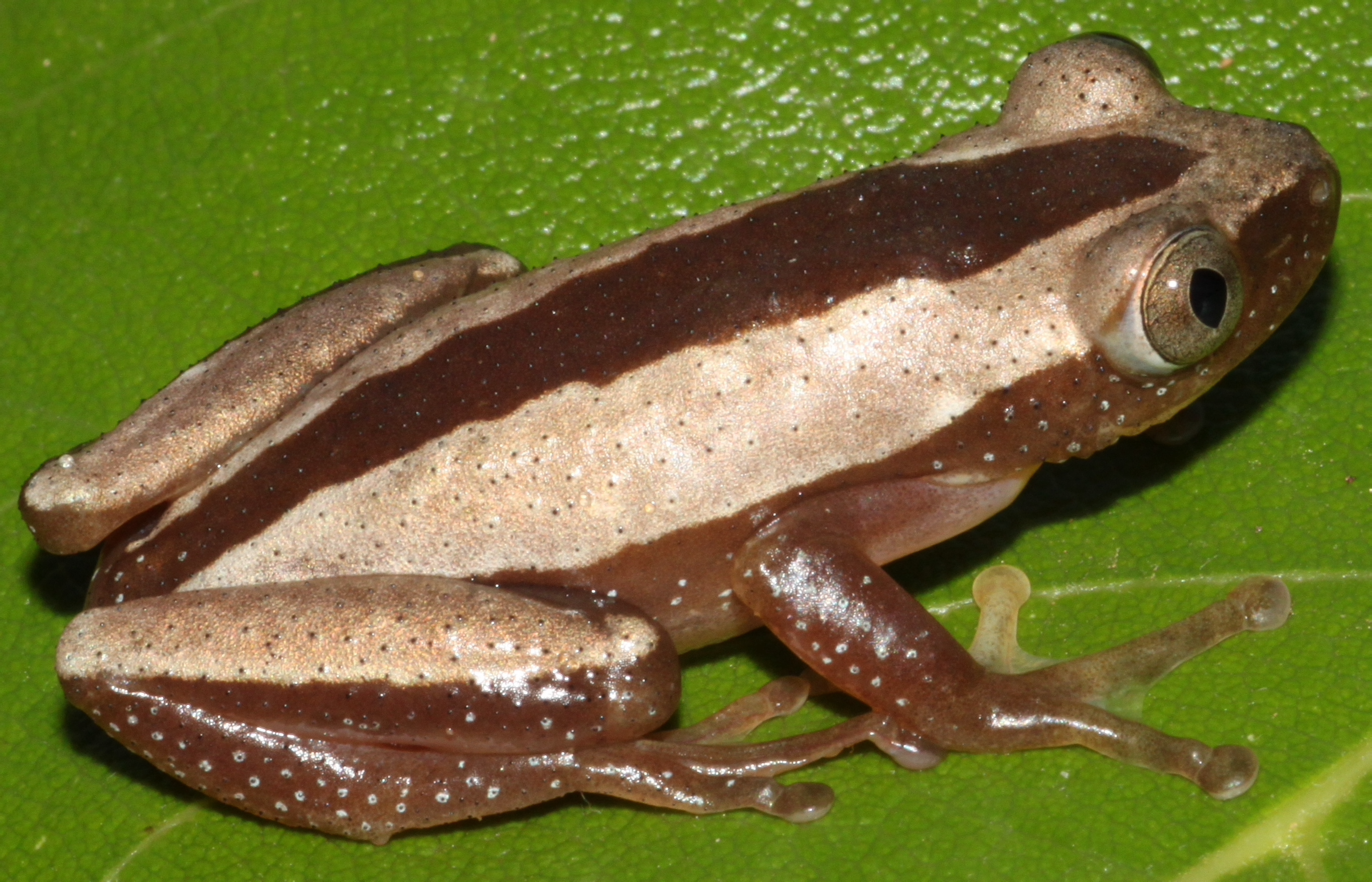
Afrixalus fornasini
To run the job and generate all outputs and final files you can simply change directory to your submit scripts and type bash ./-run_life_on_the_edge.sh-. The job will submit and you can wait for the analyses to finish (will take around 36 hours with the example data).
To look in more detail at each step and really understand what is happening throughout the LotE toolbox (recommended), follow the below procedure:
In the first part of this vignette we will perform a complete analysis of some example data for an East African spiny reed frog (Afrixalus fornasini) from start to finish. We provide example .map, .ped, .csv and params.tsv files as part of the example dataset for the LotE package. We will run through all steps of the toolbox one at a time and pause at certain parts to check outputs when decisions need to be made that affect subsequent steps. This example uses already processed genomic data from Barratt et al. (2018), using Stacks 2, with RAD-seq data for 7309 SNPs genotyped across 43 individuals
Best practice for using LotE on an unknown (novel) dataset are to run in parts and check outputs before running through the subsequent parts of the toolbox. You can do this simply by commenting out the relevant parts of the run_LOE_exposure.R, run_LOE_sensitivity.R, run_LOE_Landscape_barriers.R, run_LOE_population_vulnerability.R with a ‘#’. For example, knowledge of population structure is needed in order to select a reasonable estimate of the number of populations (k) for Genotype-Environment Association (GEA) analyses, and if this is not correctly accounted for then GEA results may be confounded by structure in the data that is unaccounted for. To address uncertainty in the GEA analyses in particular, we have adopted a simulation approach from Salmón et al. 2021. In brief, 100 simulations of the empirical data are created with randomised genotype-environment relationships, GEA analyses are performed on each of these simulations, tracking the p-values of all SNPs, and then the adaptive signal in the empirical data is determined using a user-defined significance threshold (using z-scores) for the empirical data against the simulations data to identify statistically significant SNPs that are above this. These simulation scripts work well for most of the datasets we’ve tested LOtE on (~60), but if you have a large number of SNPs (e.g. >20,000) the simulations can be prohibitively slow to run. For this reason in the latest version of the code I’ve masked out the simulations in the submit scripts, but do feel free to test them on your own datasets and let me know if anything is amiss.
We follow this best practice here, running the following components of the LotE toolbox as separate shell scripts that call the relevant software, R scripts and functions. Essentially, all analyses will be passing the relevant parameters from the Params.csv file to control each analytical step:
- Running Exposure analyses, including Species Distribution Modelling (SDM) - biomod2
- Running Sensitivity analyses, incuding GEAs - Latent Factor Mixed Models (LFMM) and RDA (Redundancy Analysis)
- Running Landscape barriers analyses, including Circuitscape modelling
- Running Population vulnerability analyses and summarising all results
All relevant details will be reported in the log file: ./-outputs-/log_files/Afrixalus_fornasini.log
8. Exposure
To run the exposure analyses, we will simply run the following code embedded in a shell script:
singularity exec ./bioconductor_3.14.sif Rscript ./-scripts-/run_LOE_exposure.R ‘Afrixalus_fornasini’
To give you an idea of what this is doing - this will read the contents of the run_LOE_exposure.R script, running through each line in sequence. The script itself sources all the internal LotE functions on lines 3-4 and then calls them on each new line. Below, you can see that each function will be passed the species name (‘species_binomial’) to run the analyses, and each internal function will extract the parameters from the relevant line of the params file that matches the species name
prepare_spatial_data(species_binomial)
prepare_environmental_data(species_binomial)
spatially_rarefy_presences_and_create_background_data(species_binomial)
sdms_biomod2(species_binomial)
exposure(species_binomial)
impute_missing_data(species_binomial)
This code will take a little while to run everything depending on your parameters, the longest step being the SDMs. Below is an overview of what is happening at each stage and which outputs are generated by each function/script:
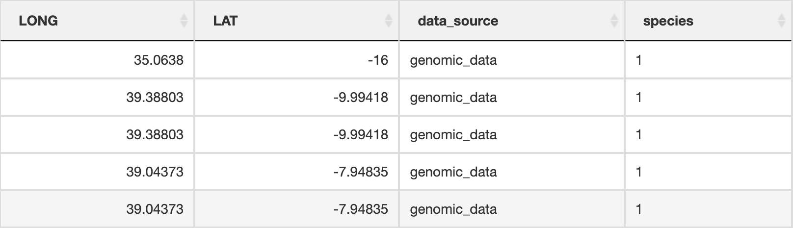
prepare_spatial_data() prepares the spatial data prior to building SDMs. The script will download existing GBIF (Global Biodiversity Information Facility) data for your defined species, and clean it using the CoordinateCleaner R package (Zizka et al. 2019). Data will be cleaned to remove any records without coordinates, those that are representing country centroids, biodiversity institutions (e.g. museums, university collections), and those that are geographic outliers from the rest of the species range (>1000km, this can be modified in the script). The cleaned GBIF data will be combined with the existing georeferenced genomic data and written as a new file ending in _presence_data.csv which will be used for spatially rarefying the presence data prior to building SDMs. The output file from this will look something like below (image truncated):
Spatial data table
prepare_environmental_data() reads the environmental data stored in the current and future directories and crops it to the geographic extent for the target species. Note that if you have set the params variable ‘env_data_download’ to ‘yes’ then Worldclim version 1 data will be auto-downloaded (based on the additional other parameters you defined for the spatial resolution, RCP scenario, GCM and year of projection, see section 1 above). This is important to ensure that SDMs in particular are modelling an area that is ecologically relevant for the study species. If the variable ‘geographic_extent’ is defined in the params file (xmin, xmax, ymin, ymax) then this will be taken as the geographic modelling extent, and if this is not populated, the function will take the extent covered by all presence samples written above by prepare_spatial_data() to define the modelling extent. Secondly, the function will then extract the relevant environmental data for all predictors at each sampling location of all individuals (= populations) and store it in a new file ending _full_env_data.csv which will be used for GEAs later. The output file from this will look something like below (image truncated):
Full environmental data table

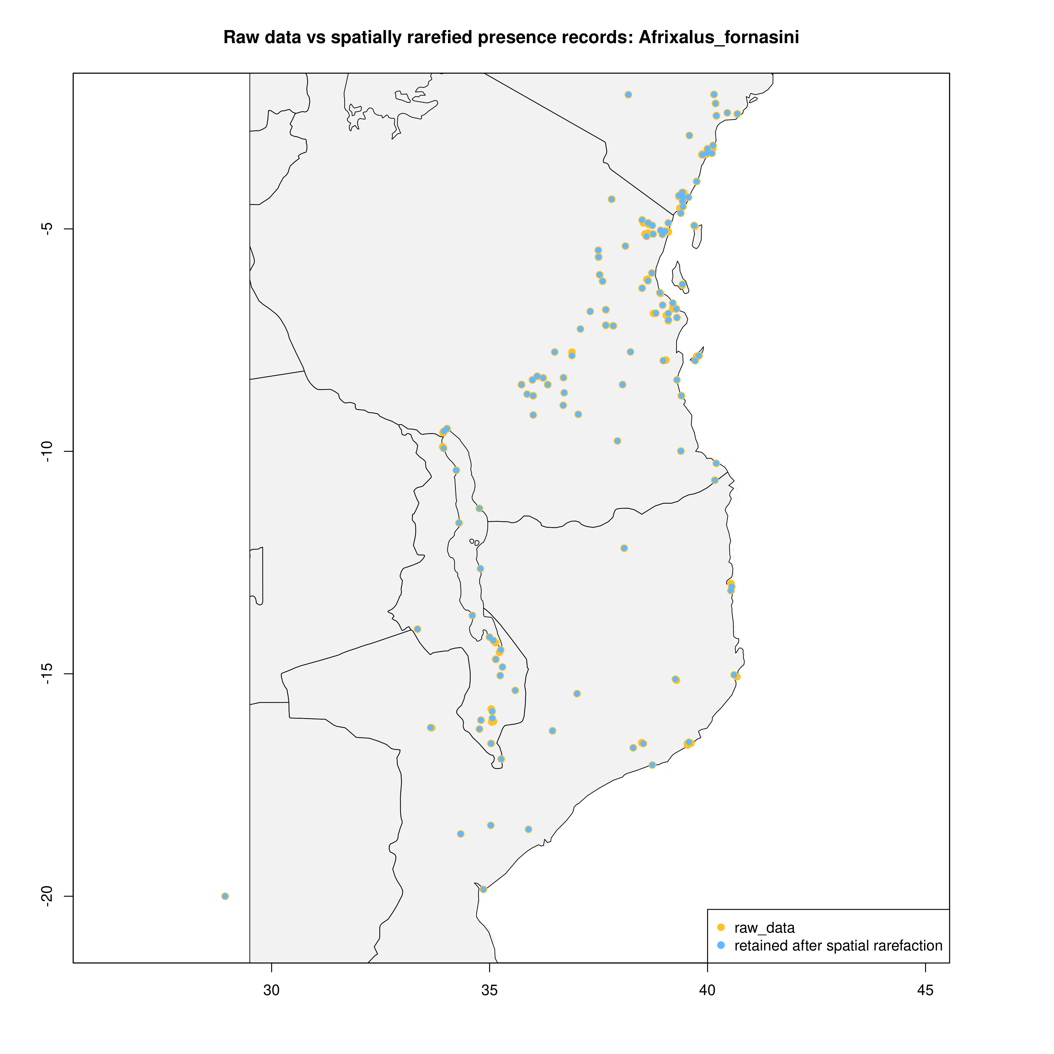
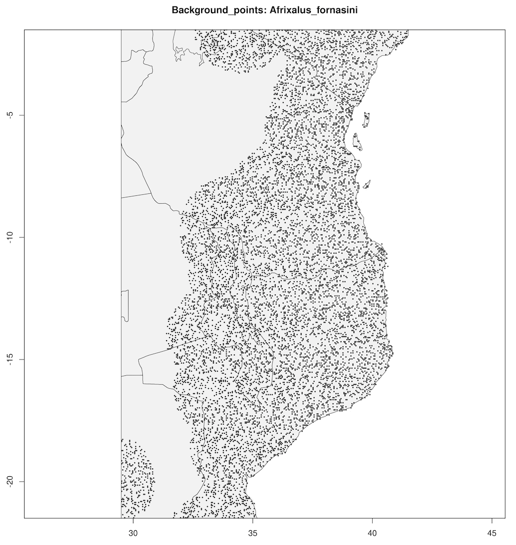
spatially_rarefy_presences_and_create_background_data() reads in the _presence_data.csv written by prepare_spatial_data() and spatially rarefies the data so that spatial autocorrelation (e.g. sampling bias) will not confound predictions made by SDMs. The ‘sp_rare_dist_km’ parameter in the params file represents the minimum distance that two presences are allowed to be, if two presences are less than this distance apart (i.e. highly spatially clustered) then one of the presences will be removed. The spatially rarefied presence data will be written as a new file (_thinned.csv) for building SDMs and plotted with the original data for visualization. The function will then generate a number of background (pseudoabsence) points from a given buffer around presence points (defined in the params file – ‘n_background_points’ and ‘buffer_distance_degrees’), writing these points as a new file (_background_points.csv) and plotting them for visualization
The output files from this will look something like below (raw data vs. spatially rarefied data and a summary of background points), and the relevant .csv files will be stored for later use by the toolbox:
Presence records
 |
Background points
 |
sdms_biomod2() will use the spatially rarefied presence data to build species distribution models (SDMs) for each species, for present conditions, but also for forecasted future conditions. Here, the framework follows SDM best practices, see Araujo et al. (2019), using reduced spatial autocorrelation in presence data, as well as accounting for multi-collinearity in predictor variables using Variance Inflation Factors (VIF) if defined in the params file. Alternatively, users may specify a subset of predictors that are ecologically relevant for the species in question (‘subset_predictors’). The biomod2 R package is used to evaluate models built using available modelling algorithms which is also subsettable via the params file, ‘biomod_algorithms’, and retaining only ‘good’ models (i.e. TSS>0.5, modifiable in the params file ‘TSS_min’ or ‘ROC_min’) for the final ensemble species distribution model prediction. If using MAXENT in your list of SDM modelling algorithms, a copy of the maxent.jar file from the MAXENT website will need to be placed in a suitable location, and this location set as the ‘maxent_path’ parameter in the params file. The model will then be projected onto the future environmental data layers to forecast the species distribution in the future. Variable importances will also be tracked across all retained models so that the user has a sense of which predictor variables have the most influence on the species distribution. Several SDM parameters are modifiable in the params file, including if VIF should be used (‘perform_vif’), or a subset of variables should be selected (‘subset_predictors’), which SDM algorithms to use (‘biomod_algorithms’), number of replicates per algorithm (‘sdm_reps_per_algorithm’, data split percentage between model training and testing (‘data_split_percentage’). The function will create a self-contained analysis subfolder within the SDMs folder containing all the models and data, summarizing the models themselves as well as various metrics of their performance
The output files from the SDMs will look something like below (current and future SDM predictions, variable importances of model predictors and overall performance of different modelling algorithms that passed defined thresholds to generate final ensemble models)
Current and future SDMs
Variable importance
SDM algorithm performance
exposure() compares how SDM predictions change between the present and predicted future conditions. It takes this information and uses it to calculate ‘Exposure’ (ranging from 1-10), measuring the magnitude of change each population/locality will experience between the two time periods. The output files from the exposure analysis will look something like below (predicted change between current and future SDM predictions – range expansions in green and range contractions in orange)
Environmental dissimilarity plot
From these data, a final Exposure.csv file will be generated that summarises all the changes in the SDM and your selected environmental predictors for each population (i.e. unique LONG/LAT)
Environmental dissimilarity table

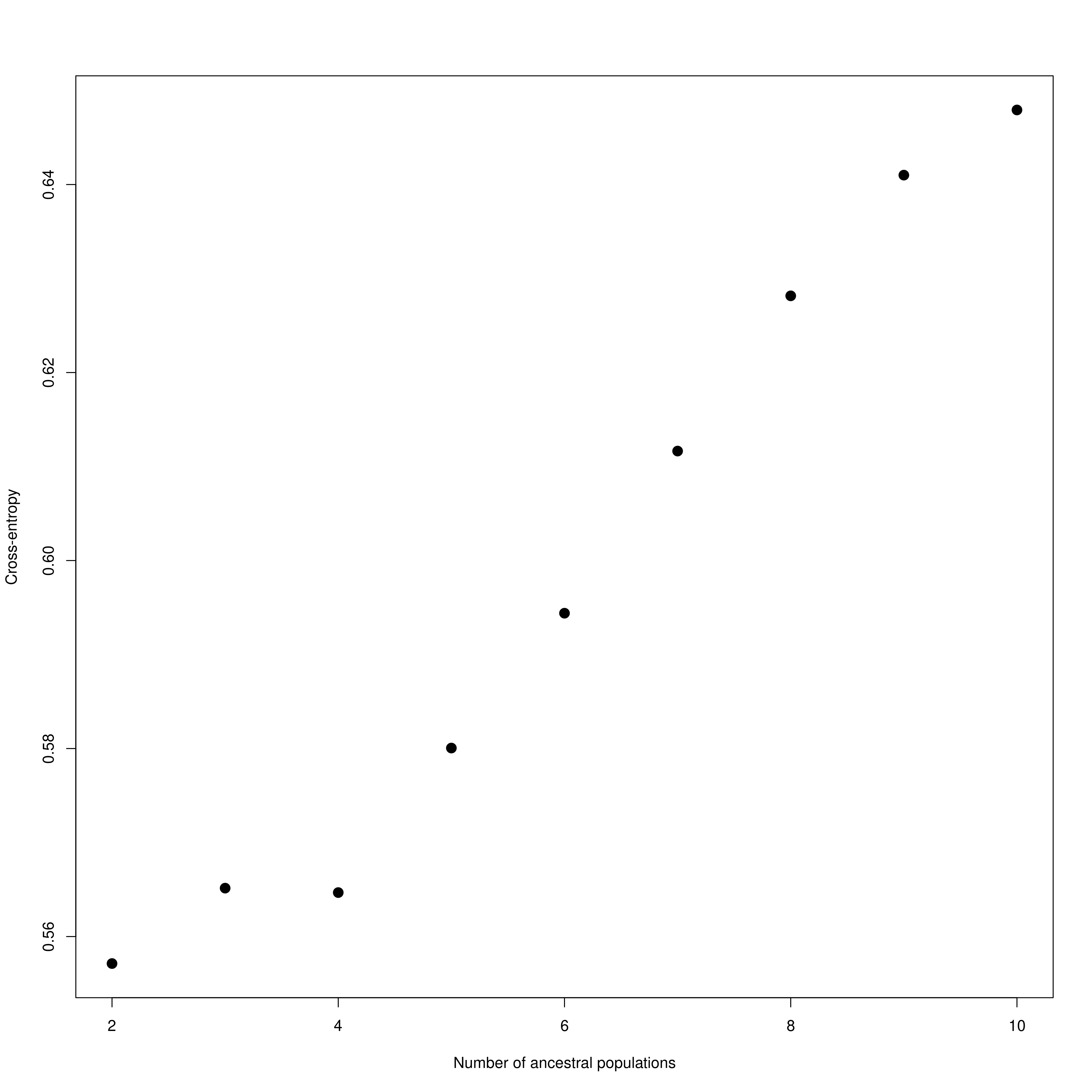
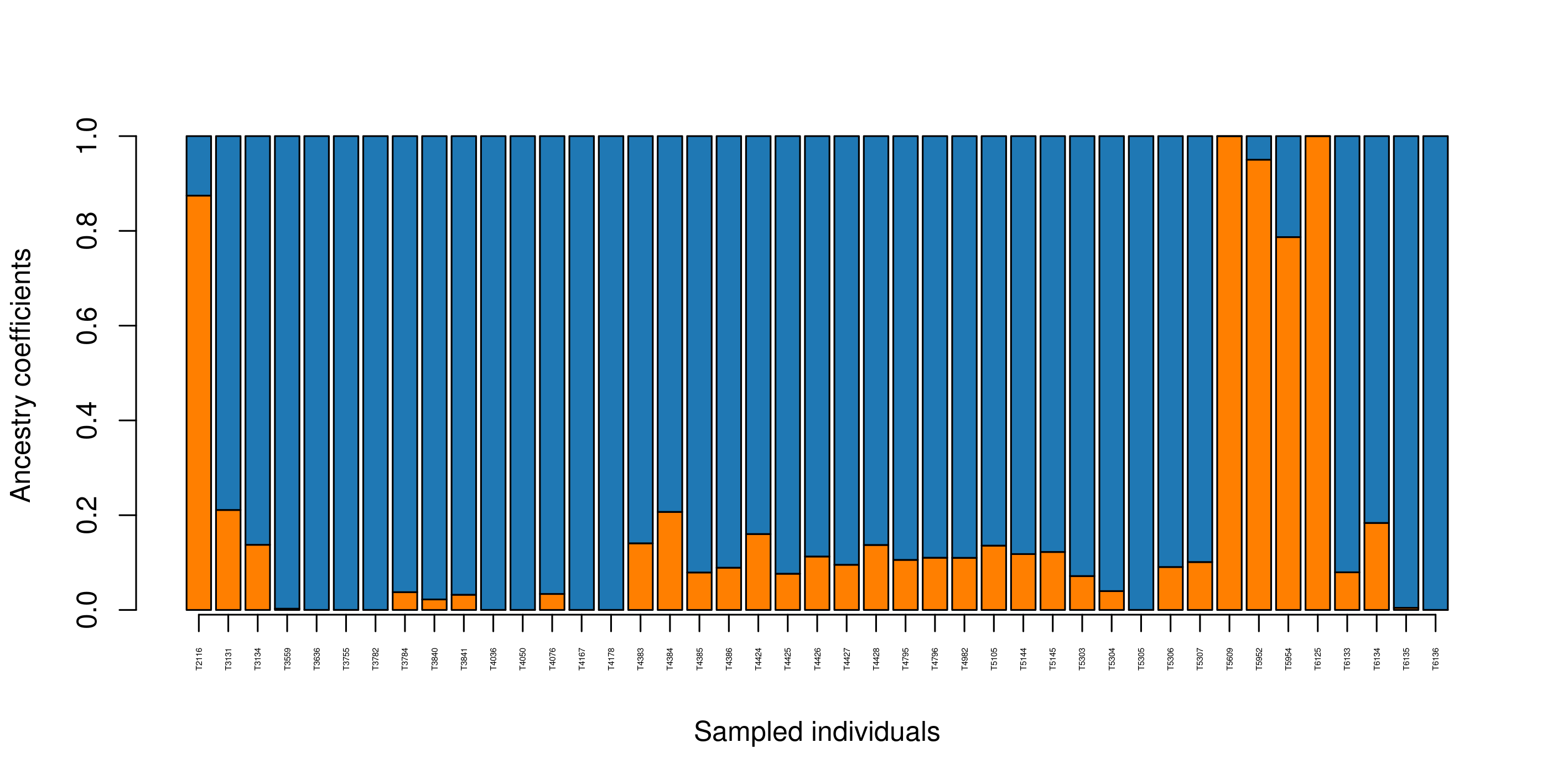
impute_missing_data() A final step of the ‘Exposure’ submit script is to set up files for the next step (‘Sensitivity’). Firstly, because GEA analyses (LFMM and RDA) typically require complete data matrices of called SNP genotypes, something which is not achievable using reduced representation library approaches (e.g. RAD-seq/ddRAD-seq), it is necessary to impute missing data, which will be done in two ways, firstly using LEA (Frichot & François 2015), and secondly based on the mean frequencies of genotypes per population cluster (see Razgour et al. 2018). This will generate additional files (_imp.csv, _imp.geno and _imp.lfmm) in the -data-/genomic_data/ directory for use with the GEA methods in the next part of the toolbox. Lastly, some basic population structure analyses will be performed in order to understand the spatial population structure of the data so that the GEAs are accounting for this. This will be performed as part of this function and will be output in the -outputs-/genomic_analyses/ folder – with a _pop_structure_pca.png file (including a PCA plot of the data and the inertia of each PC axis) as well as an _snmf_barplot.png and _snmf_cross_entropy.png file which together can be used to determine likely structure. The output files will look like below, with a PCA plot and inertia of each PC axis, a summary of the cross-entropy values for varying values of k specified in the params file, and a barplot of the population structure selected by the best k
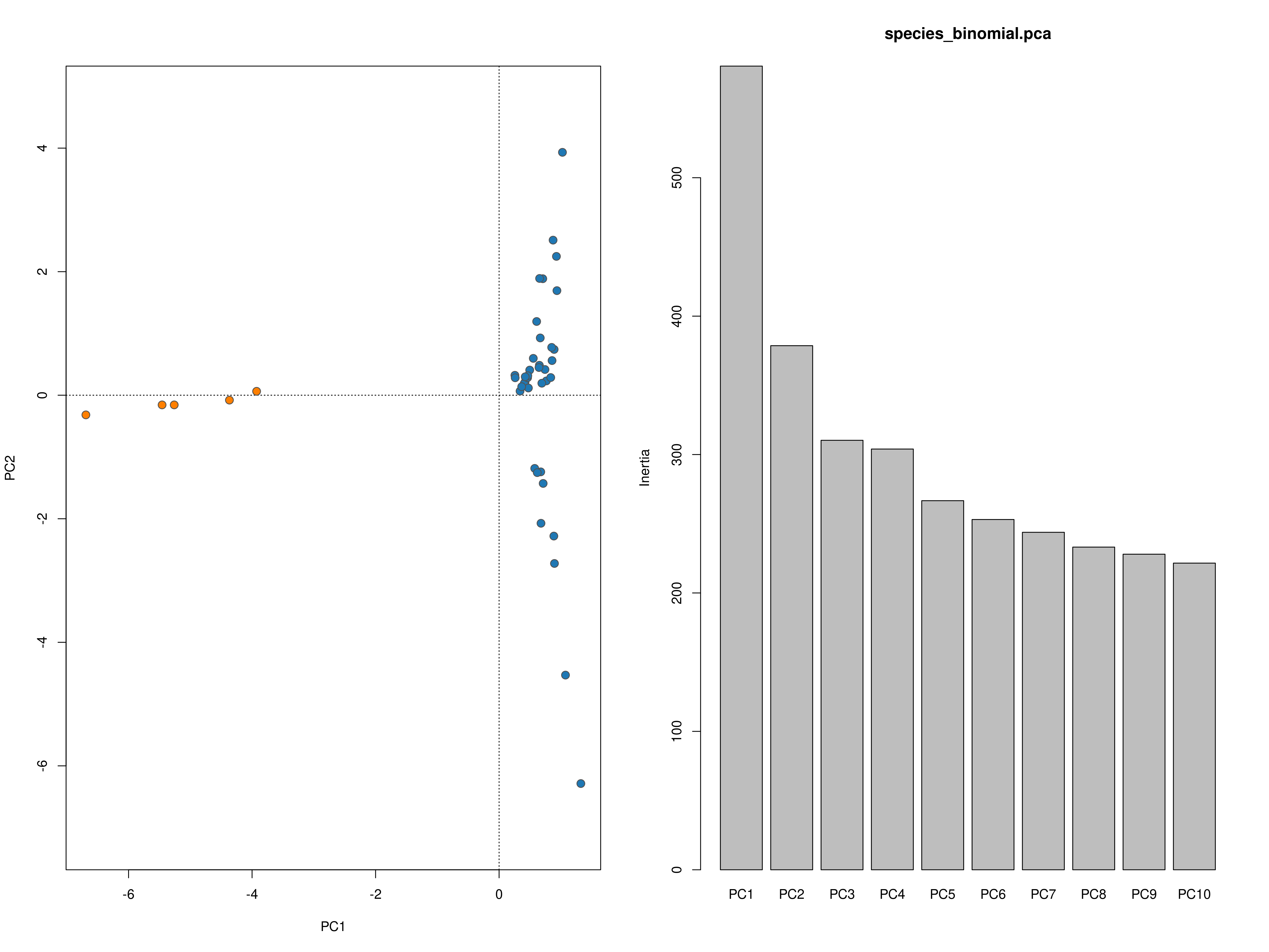
Population structure PCA
Population structure
 {:.image-caption}
Population structure sNMF barplot
{:.image-caption}
Population structure sNMF barplot
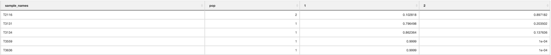
Finally, a population assignment file is made (_pop_assignment_LEA.csv) which has the population assignment for each individual:
Population assignment
At this point it is important to update the params file for your species with the most appropriate number of population clusters represented in the data (‘k’).
9a. Simulation and sensitivity analyses for GEA (local adaptation) analysis
Before blindly ploughing ahead with Sensitivity part of the LotE Toolbox, we highly recommend exploring the potential adaptive signal in the data first, using our simulation scripts. The below code, embedded in a shell script will first explore a range of parameters for the GEA (LFMM and RDA) analyses on your dataset, demonstrating the sensitivity of the False Discovery Rate threshold (for LFMM) and the Standard Deviation (SD) from the mean loadings (for RDA). It will create a plot of the number of SNPs identified as candidates under selection and their false positive (FP) rates for each of your predictors for both LFMM and RDA analyses. A great resource for understanding this more can be found here and here. Obviously, for LFMM analyses - as FDR is increased, you will recover more candidate SNPs but these may be potential FPs. Similarly, for RDA analyses reducing the SD from the mean loadings will recover more candidate SNPs which again may be potential FPs. A good rule of thumb is to examine the output plots to gauge what you are comfortable with in terms of numbers of SNPs vs. FPs, selecting the most appropriate value of FDR and SD for your real LFMM and RDA analyses. These can then be set in the params file (‘lfmm_FDR_threshold’, and ‘rda_SD_threshold’).
singularity exec ./bioconductor_3.14.sif Rscript ./-scripts-/simulations/-00_parameter_exploration-.R ‘Afrixalus_fornasini’
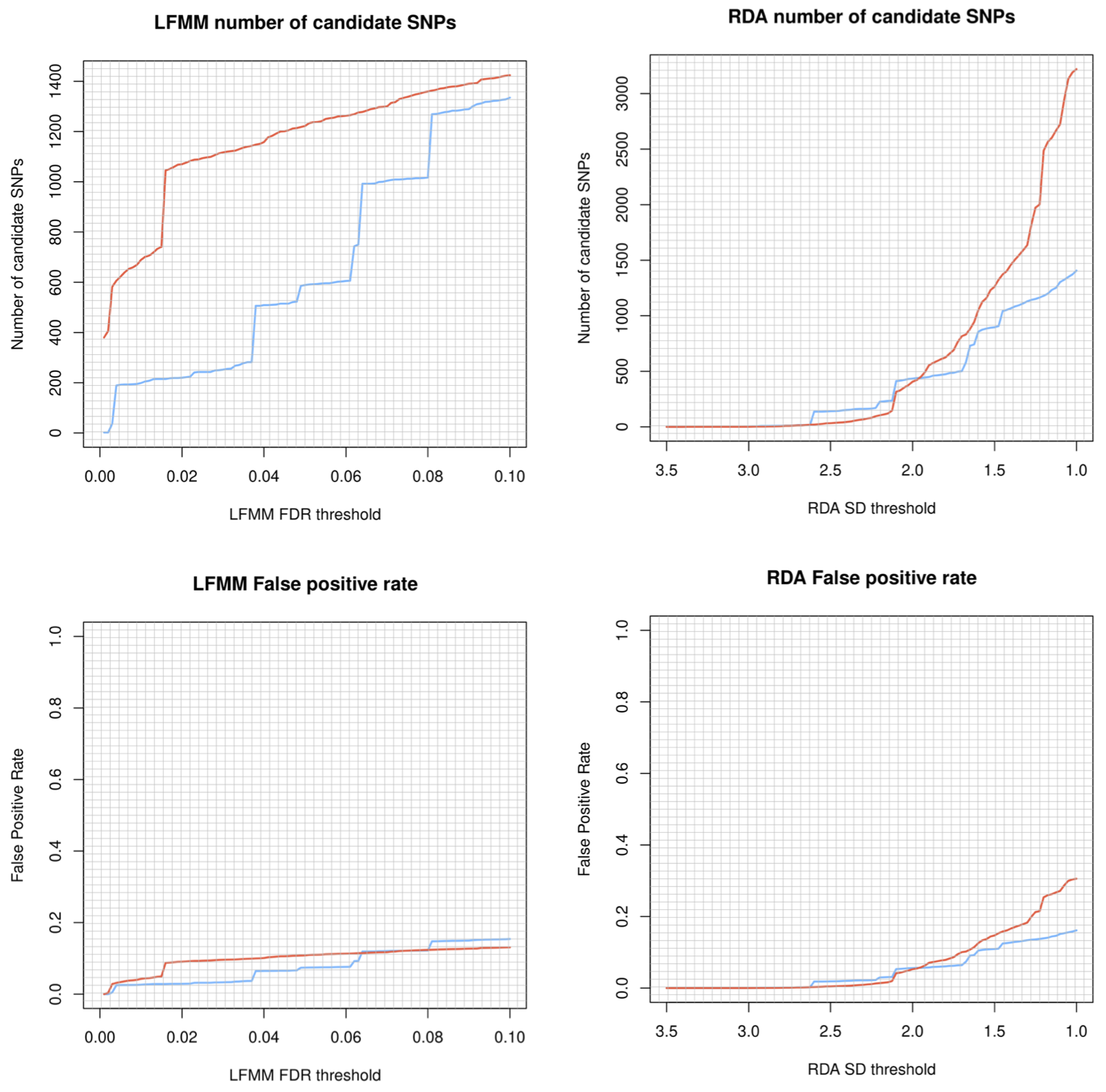
LFMM and RDA sensitivity
Once you have an idea of the optimal parameters for RDA and LFMM analyses, you can then press on with those analyses. By running the below code, the LFMM and RDA analyses will be performed, firstly to generate empirical results from your data (using the -01_empirical_data-.R script) based on the parameters you supplied in the params file ((‘lfmm_FDR_threshold’, and ‘rda_SD_threshold’).
Next, we will use simulations to test the validity of the adaptive signal in your empirical results following the approach of Salmón et al. 2021. The -02_randomise_data-.R script will generate 100 permutations of the datasets, with randomised genotype-environment associations (you can think of this as a permutation test). After this, the -03_perform_simulations-.R will perform LFMM and RDA analyses on each of these 100 simulated datasets. Lastly, the -04_evaluate_significance-.R script will extract all of the p-values for all SNPs in your dataset across the empirical data and all 100 simulations, and by determining a significance threshold (e.g. as the 95th percentile of the Z-score distribution) will categorise candidate SNPs from the empirical analyses above this threshold as significant. A plot will then be created of the identified candidate SNPs in LFMM and RDA analyses, with an adjacent colour-coded plot next to them to indicate if the relevant candidate SNP is statistically significant (green), or non-significant (orange).
singularity exec ./bioconductor_3.14.sif Rscript ./-scripts-/simulations/-01_empirical_data-.R ‘Afrixalus_fornasini’
singularity exec ./bioconductor_3.14.sif Rscript ./-scripts-/simulations/-02_randomise_data-.R ‘Afrixalus_fornasini’
singularity exec ./bioconductor_3.14.sif Rscript ./-scripts-/simulations/-03_perform_simulations-.R ‘Afrixalus_fornasini’
singularity exec ./bioconductor_3.14.sif Rscript ./-scripts-/simulations/-04_evaluate_significance-.R ‘Afrixalus_fornasini’
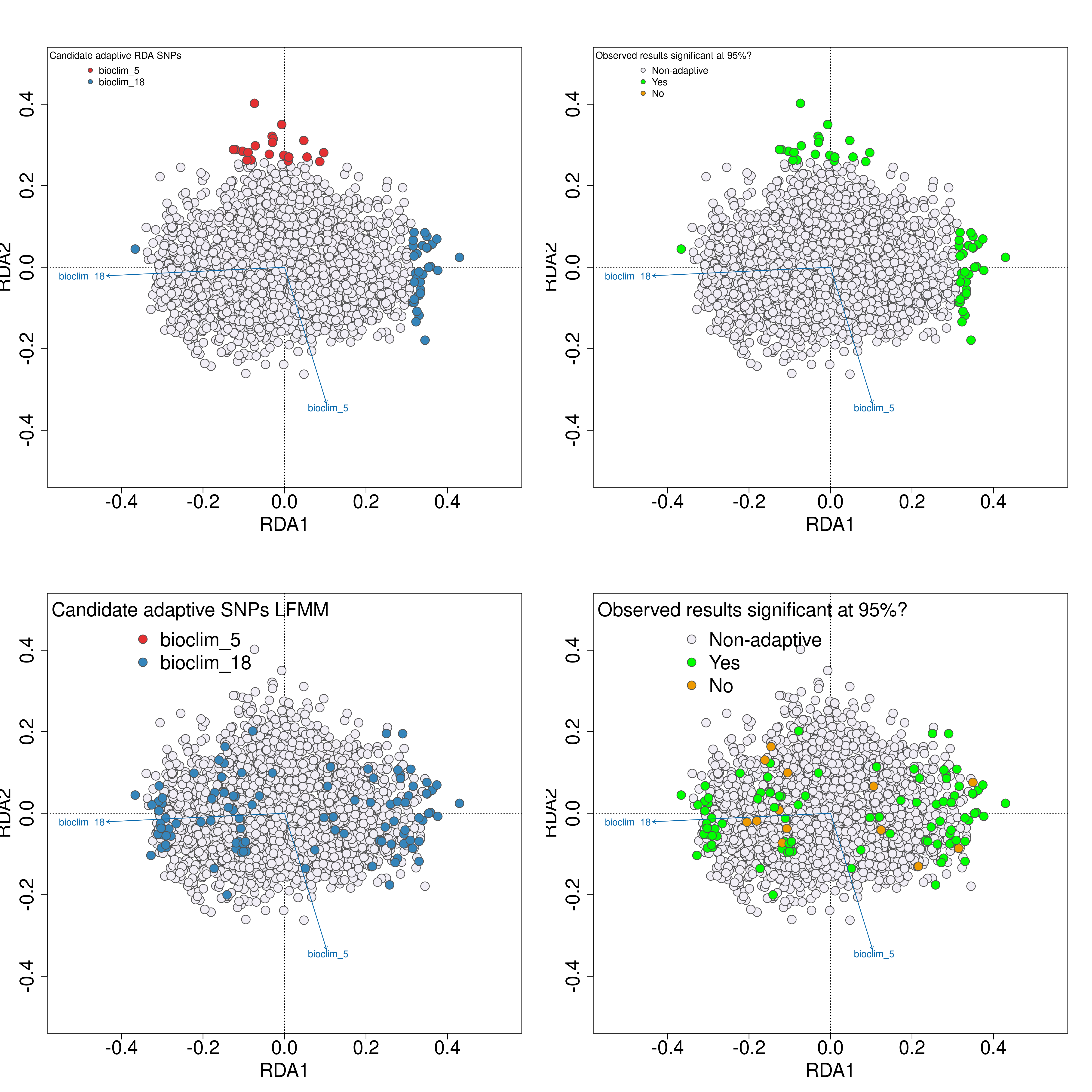
Validation of candidate SNPs based on simulations
The simulation scripts above will generate a text file with a list of all of the statistically validated candidate SNPs, named ‘Afrixalus_fornasini_adaptive_loci_validated.txt’. If this file exists (i.e. if you have run all the sensitivity analyses), this file (rather than the standard [unvalidated] ‘Afrixalus_fornasini_adaptive_loci.txt’ will be used to perform the local adaptation analyses - specificially for quantifying genomic offset and quantifying local adaptations.
09b GEA- LFMM
The following sections (09b and 09c) provide more detail on the LFMM and RDA analyses which have been performed in the sensitivity and simulation analyses described above. These sections may be less relevant to read deeply into if you have performed the simulations and sensitivity analyses and are confident on the list of candidate SNPs that you have
LFMM is a univariate method that will account for population structure from the underlying data, and SNP genotypes will be statistically evaluated against your defined environmental predictors to select candidate SNPs that are potentially under selection. LFMM will read in the environmental data you prepared using prepare_environmental_data(), and subset the variables of choice (defined as ‘env_predictor_1’ and ‘env_predictor_2’ in the params file). As highly colinear variables are problematic for GEA it will check the Variance Inflation Factor and report the correlation between the variables in a pair plot (_env_correlations.png). If your variables are highly correlated (e.g. >0.8) it may be worth considering alternative variables from your predictor set that are less strongly correlated
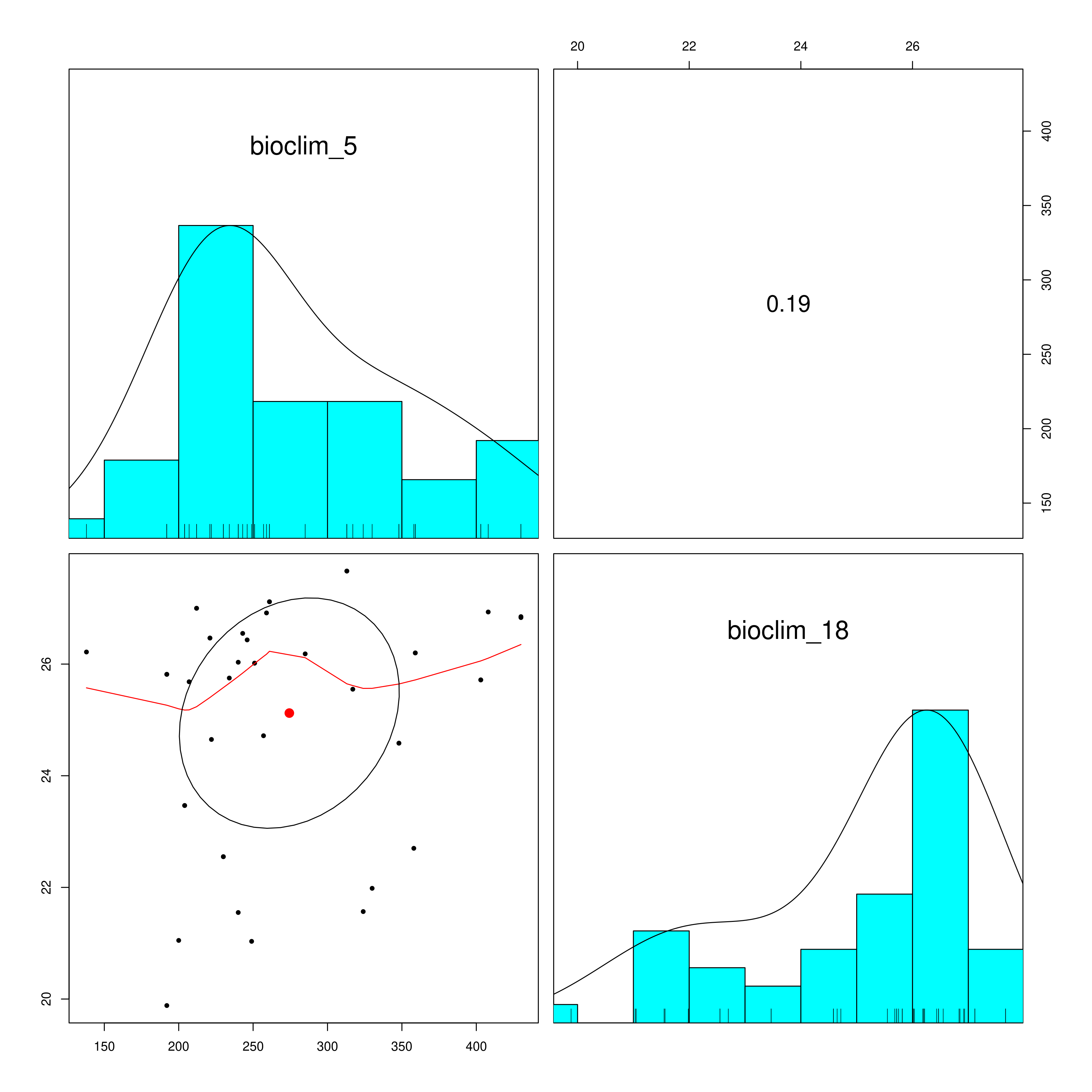
Environmental data correlations
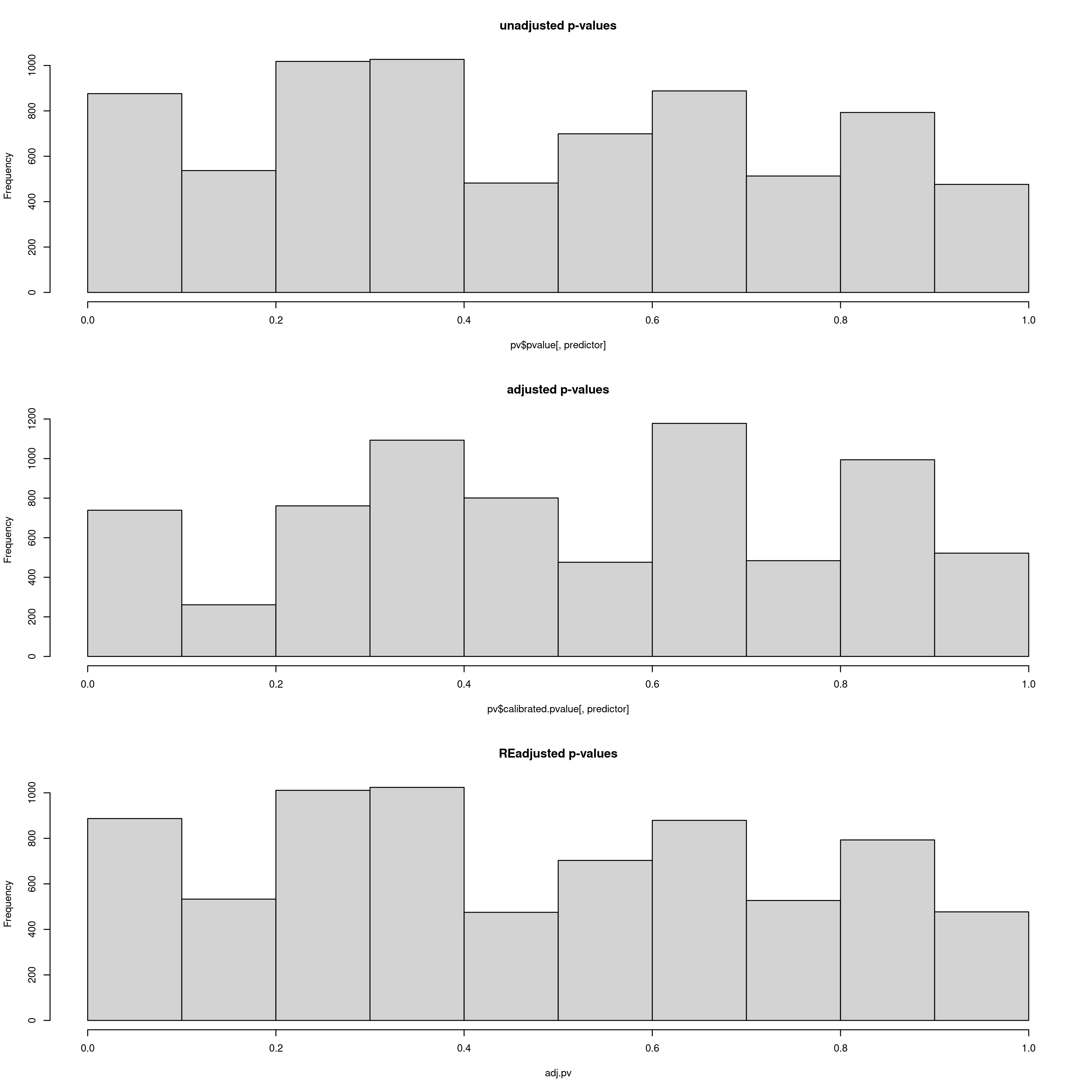
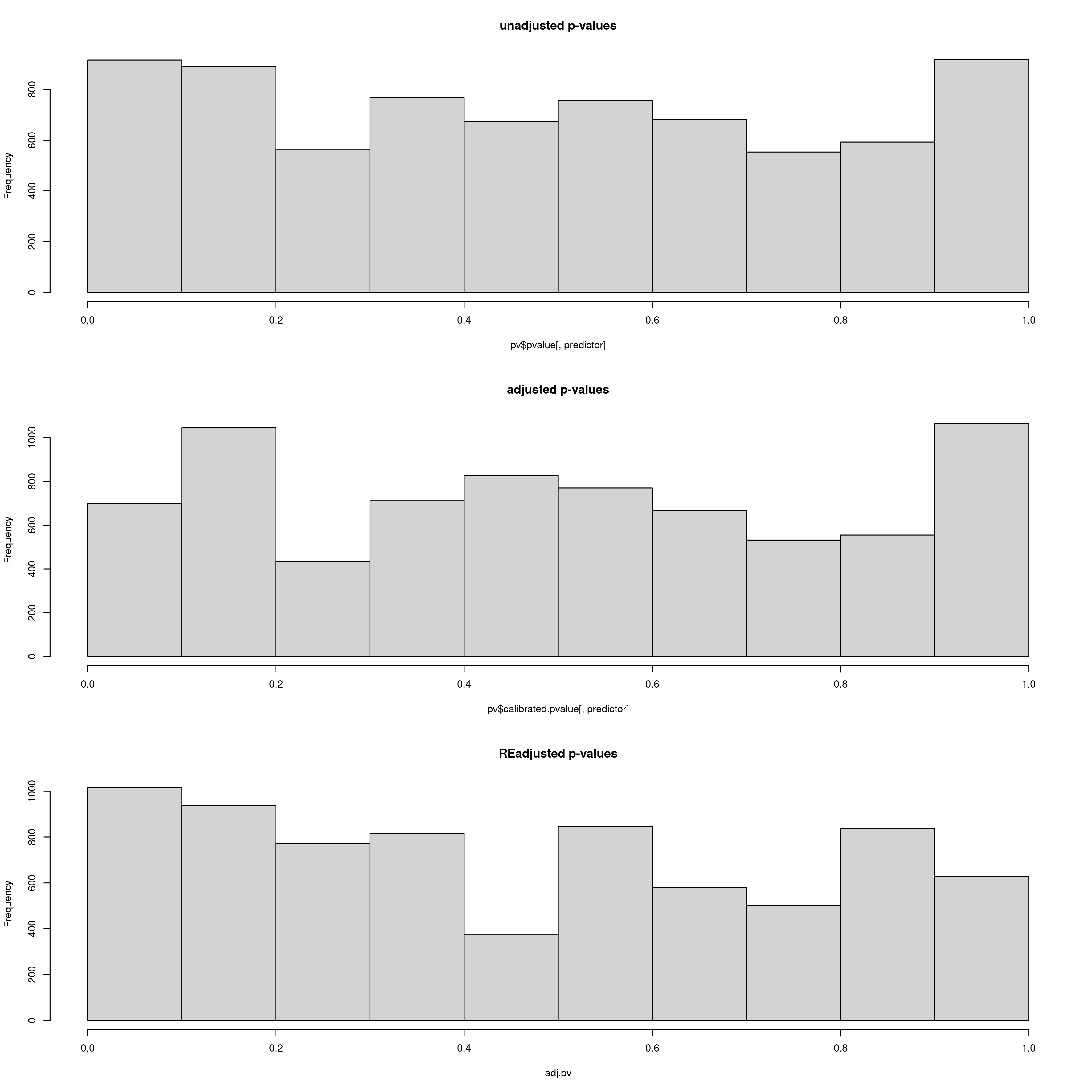
After this step, the data will be analysed using LFMM (reading your newly populated value of k from your params file). LFMM will read the imputed LFMM formatted file (the one generated by impute_missing_data()), and perform a GEA to search for candidate SNPs that show strong statistical correlations with your environmental predictors. For each SNP, a p-value will be assigned, which will be used to calculate a q-value. This q-value will ultimately be used to decide which candidate SNPs pass the pre-defined FDR (False Discovery Rate) thresholds of 0.1, 0.05 and 0.01 by default, but if you are running the simulation scripts before this stage, there will be a greater number of FDR rates. Firstly the p-values and calibrated p-values will be calculated, and then the GIF (Genomic Inflation Factor) will be used to rescale the p-values into an acceptable distribution. We recommend that the ‘scale_gif_lfmm’ parameter in params be set to 1 (i.e. no scaling) on first running LFMM, but see this great tutorial on GIF modifcation in LFMM for more details if you want to investigate further. The LFMM script will summarise the p-values, the calibrated p-values and the scaled p-values so that you can look at their distributions. Ideally you want a histogram distribution more leaning towards the left (i.e. low p-values), but not too liberal (i.e over-representative high frequencies of low p-values). The plot should be investigated to ensure an acceptable p-value distribution (i.e. not to conservative, not too liberal).
Output plot of p-values, calibrated p-values and re-adjusted p-values. Here the re-adjusted p-values after modifying the GIF using the scale_gif_lfmm parameter in the params file look acceptable, so we will go with this for now
Bioclim 5 p-value distrubtions for LFMM analyses
Bioclim 18 p-value distrubtions for LFMM analyses
You may experiment with the GIF, running LFMM a few times until you are satisfied with the readjusted p-value distributions (lower panel). In the log file, the GIF is reported each time, so you can use this to adjust the ‘scale_gif_lfmm’ parameter which modifies the GIF. A well calibrated set of p-values should show a GIF of around 1, too liberal <1 and too conservative >1, so if your GIF is around 1.8 for example, and your p-values are very skewed towards high values, you could set your ‘scale_gif_lfmm’ parameter to 0.7 which would bring the newly calculated GIF to 1.26 (=1.8 x 0.7) and increase the frequency of lower p-values. Each time, your list of candidate SNPs that are selected to be below the defined FDR (False Discovery Rate) thresholds (0.1, 0.05, 0.01) will change, and it is worth keeping in mind that only a fraction of your total loci (in this case the total is 7309) should realistically show signals of local adaptation. Thus, histogram distributions that are too liberal will detect high numbers of false positives, and too conservative approaches will result in zero detections. P-values are often not well behaved in empirical datasets so you should modify the GIF to an extent that the numbers of candidate SNPs and their p-value distributions are tolerable for you and believable for your study species – there is no right or wrong way to do this, it is subjective, and as long as you report your criteria exactly it is perfectly acceptable. In this regard, the simulation scripts may go soome way to helping you decide what is acceptable for your study system.
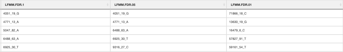
The output files containing your candidate SNPs will be written per predictor and also summarized in _LFMM_candidate_SNPs.csv (truncated file below). The numbers of SNPs below each FDR threshold will be reported in the log file
LFMM candidate SNPs
After LFMM has completed and you are satisfied with your candidate SNPs, we will proceed with running RDA before performing the rest of the ‘Sensitivity’ analysis, which is somewhat less convoluted
09c. GEA- RDA
Similar to LFMM, RDA (Redundancy analysis), a univariate method, will be implemented using the vegan package in R. The process is similar to LFMM whereby population structure will be accounted for in the underlying data, and SNP genotypes will be statistically evaluated against your defined environmental predictors to select candidate SNPs that are potentially under selection. The RDA method implemented here applies the same framework as LFMM, whereby the GIF can be adjusted (using the ‘scale_gif_rda’ parameter) to select thresholds for candidate SNPs, but it will also select outlier candidate SNPs using a function that measures the standard deviation of each SNP from the mean loading value across all SNPs (Razgour et al. 2019). We recommend setting this standard deviation (‘rda_sd’) in the params file to 2.5 by default, but you can make this threshold more conservative (e.g by setting it to 3)
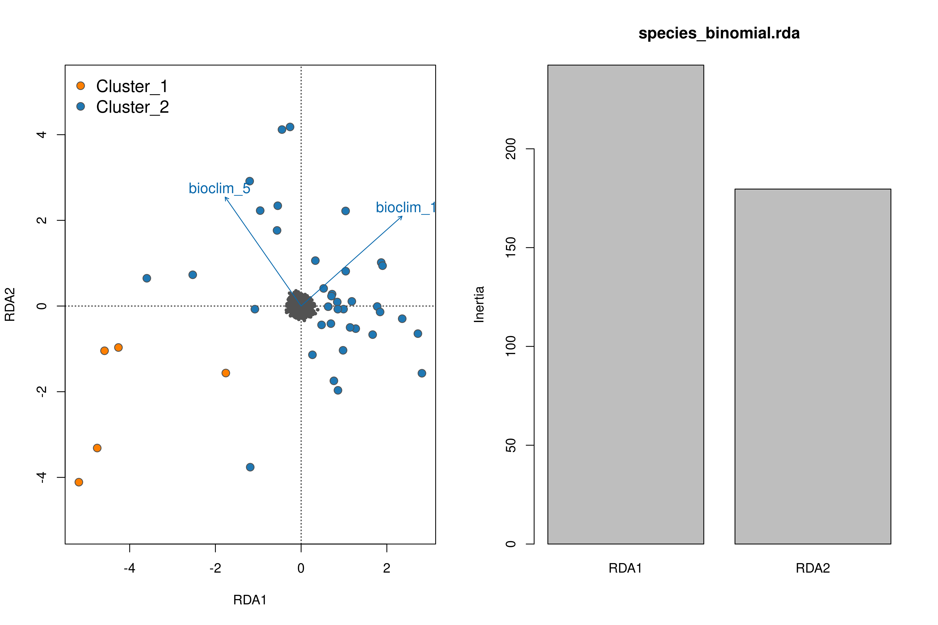
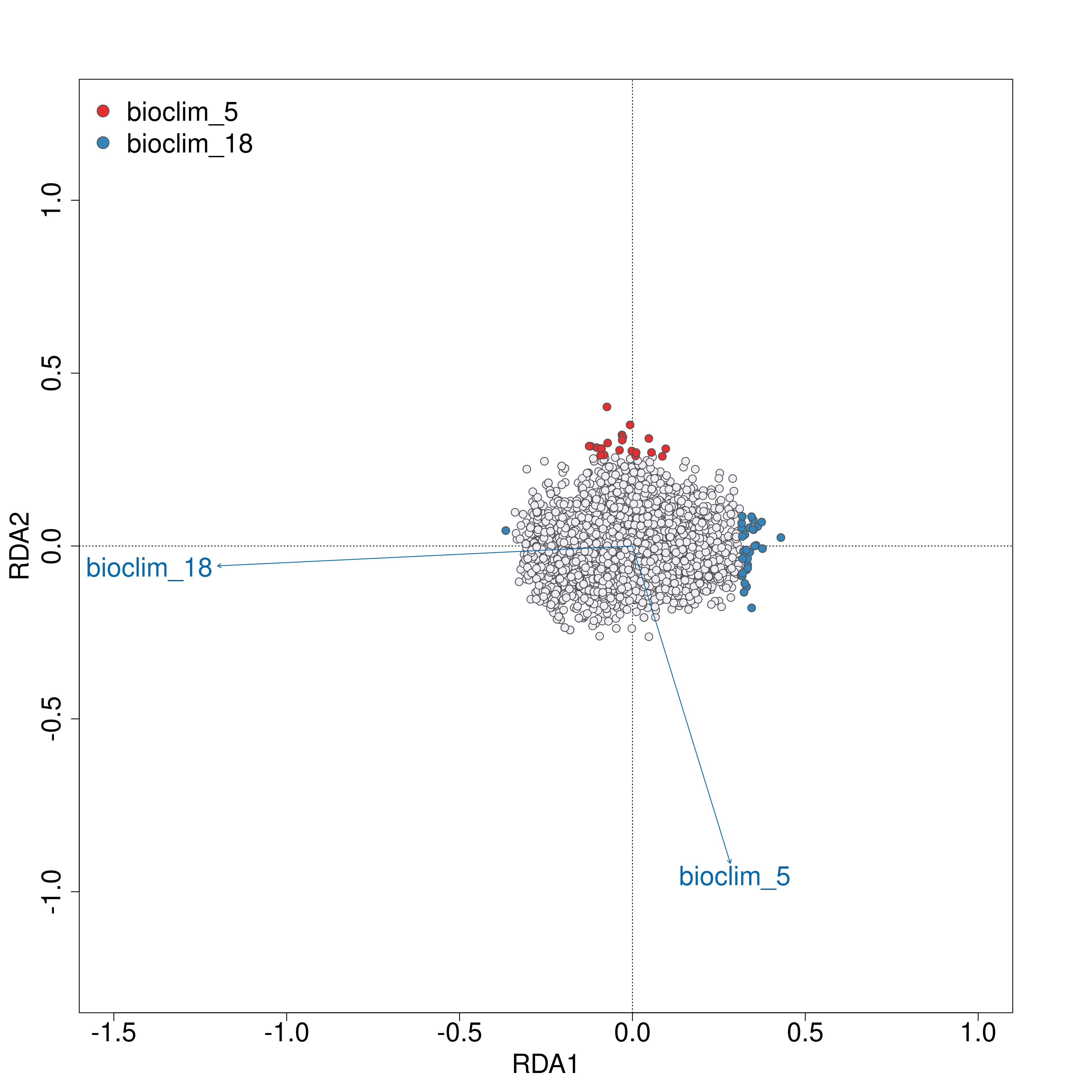
Once the RDA script has run you can investigate the outputs; of particular interest here is the first plot (_RDA_plot.png) which will show in the left panel the clustering of individuals in ordination space and their position relative to the biplot arrows of each predictor, and in the right panel will show the eigenvalues of the PC axes
RDA plots
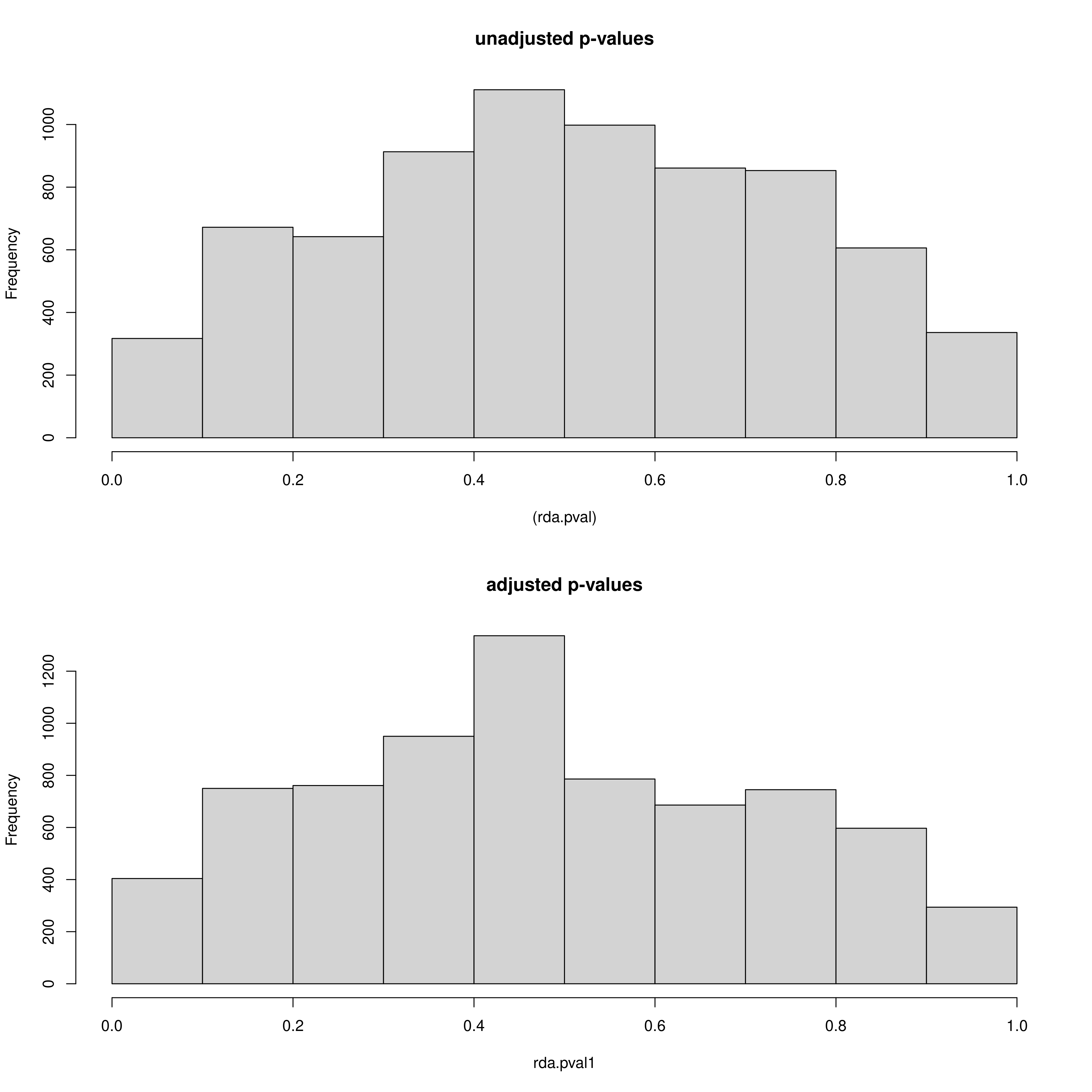
Secondly, just like with LFMM we can see the histogram of the unadjusted and adjusted p-values (after modifying the GIF) of the SNPs, but this time for each predictor (_RDA_p_value_distribution_env_1.png, _RDA_p_value_distribution_env_2.png). Like with LFMM, the distributions of these p-values can be modified by updating the GIF (‘scale_gif_rda’) in the params file and rerunning the script
RDA p-value distributions
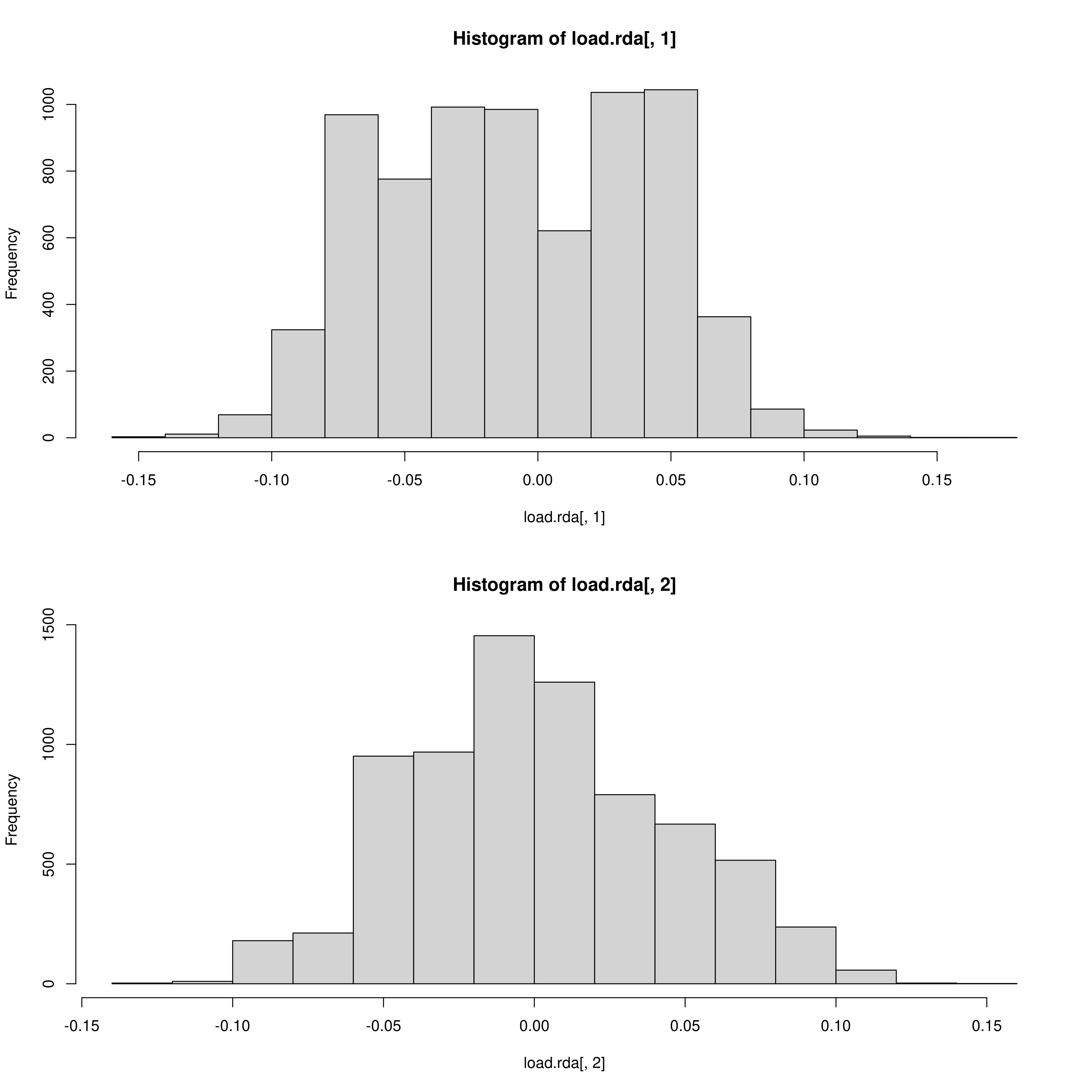
The outlier approach to selecting candidate SNPs is also adjustable as mentioned, outputting a two panel (i.e. a panel for each environmental predictor) histogram of the loadings of each SNP in the dataset. The outer head and tails of the distribution are classed as outlier candidate SNPs (defined using the ‘rda_sd’ parameter in params)
RDA histogram of loadings
RDA candidate SNPs
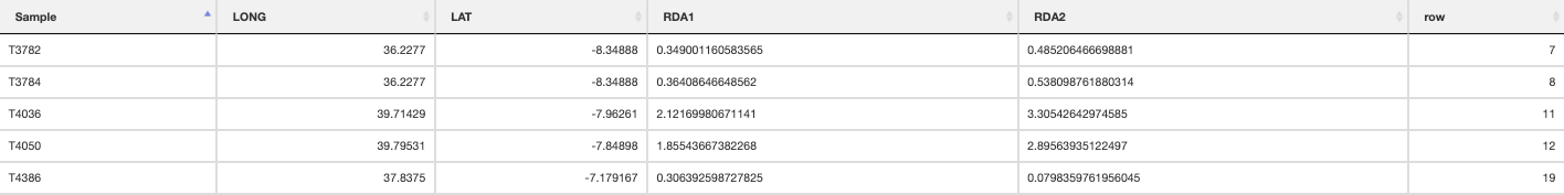
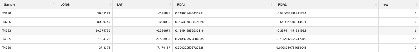
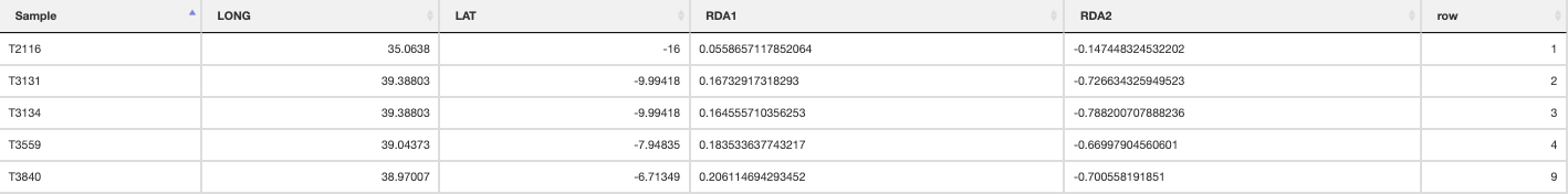
An output plot of the SNPs in the RDA ordination space coloured by their environmental predictor association will be made (outlier approach using standard deviation). A list of all candidate SNPs across the different FDR thresholds (<0.1, <0.05, <0.01) will be also be made for each predictor
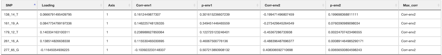
RDA list of candidate SNPs
10. Sensitivity
If you are satisfied with the LFMM and RDA analyses (having explored how changing the GIF and/or standard deviation parameters affects the output candidate SNPs), we can continue with the rest of the analysis. To continue with the rest of the ‘Sensitivity’ analysis, we submit the following code embedded in a shell script:
singularity exec ./bioconductor_3.14.sif Rscript ./-scripts-/run_LOE_sensitivity.R ‘Afrixalus_fornasini’
Again, to elaborate what this is doing - this will read the contents of the run_LOE_sensitivity.R script, running through each line in sequence. Again it will pass the species name to each of the functions and run them line by line:
gea_lfmm(species_binomial)
gea_rda(species_binomial)
gea_individual_categorisation(species_binomial)
quantify_local_adaptations(species_binomial)
genomic_offset(species_binomial)
neutral_sensitivity(species_binomial)
adaptive_sensitivity(species_binomial)
create_circuitscape_inputs(species_binomial)
gea_rda(species_binomial) and gea_lfmm(species_binomial) will re-run the RDA and LFMM analyses with your ‘optimised’ parameters (defined in the params file, see section #9 above).
gea_rda_individual_categorisation(species_binomial) categorises each individual based on their relative position in the constrained RDA ordination space relative to the environmental predictors (see Razgour et al. 2019). The script automatically reads in putative candidate SNPs that have been identified by either/both LFMM and RDA (definable in params file, see below) and then performs a new RDA based on only these candidate SNPs and the environmental data. Note here that if you have used the skip_gea option, then LotE will expect a space delimited file with a list of identified adaptive loci (which you presumably have prepared outside the toolbox). See section 17 for where LotE expect this file.
To select which SNPs you wish to retain for the individual categorization analysis (we recommend using option 0 to use only statisticlaly validated SNPs if you have performed the simulation analyses), set the ‘which_loci’ parameter in the params file to one of the following:
- 0: statistically validated loci only (based on the simulations)
- 1: present in either RDA (SD<3) or LFMM (FDR<0.05)
- 2: present in either RDA (FDR<0.05) or LFMM (FDR<0.05)
- 3: only LFMM loci (FDR<0.05)
- 4: only RDA loci (SD<3)
- 5: only RDA loci (FDR<0.05)
- 6: present in both RDA (SD<3) and LFMM (FDR<0.05)
- 7: present in both RDA (FDR<0.05) and LFMM (FDR<0.05) - not recommended, often 0 loci
It will write these loci to a file named _adaptive_loci.txt (see below) and use this as a basis to categorise individuals using RDA. Alternatively if you have set which_loci to ‘0’, a similar (possibly reduced list) will be used based on statistically-validated loci only.
34009_67 57923_8 16479_6 162463_8 4051_19 4771_13 6488_63 6925_30 9316_27 11941_25 13041_119 13138_107 13337_13 15727_174 16586_33 18746_22 19277_39 19464_18 21260_53 21886_17 23321_15 23671_20 27661_48 28618_16 30063_3 33339_7 33665_53 37738_33 41965_92 41986_16 41998_7 42783_178 43879_168 45109_32 46607_18 46937_27 47060_22 48682_19 48866_17 51645_31 54786_21 54805_18 56179_127 56521_18 56814_22 58602_22 60566_53 64252_19 65167_6 65398_16 68651_14 69485_46 71866_18 73357_8 73366_52 77814_42 79456_58 79823_19 81237_6 81502_137 81968_25 82779_31 83107_60 84730_74 84940_7 88620_16 88692_16 88887_11 91354_149 91712_18 92066_58 92391_65 95366_11 95672_6 96269_118 98767_76 99548_11 100156_6 104504_77 105945_66 106808_10 107851_43 108520_8 108760_75 109876_32 110024_8 114097_64 116688_10 121595_26 121776_57 124470_112 128427_45 131649_14 131965_19 132281_6 133641_28 134098_42 135668_6 139297_11 141170_23 143267_117 150670_137 156487_12 169030_35 172684_21 178281_42 182134_11 187259_14 192959_11 196422_15 198685_148 211039_81 213940_114 217781_180 218174_45 225052_17 225728_8 234703_45 235389_31 238471_154 249414_20 249640_39 253409_48 253429_61 261805_105 262660_38 268195_20 269752_51 273209_151 273904_105 274346_9 293532_8 295658_7 355497_49 374443_18 394672_17 407884_17 522712_33 589433_21 628214_19 740461_10 818212_24 880025_111 938469_59 960865_51 3065_8 6249_20 13129_29 13630_19 16341_9 16479_6 26646_6 30809_29 36954_12 41441_56 54749_17 56639_59 57827_91 57923_8 59161_54 66570_7 74287_14 76417_25 77016_7 77412_10 79773_24 80819_8 89524_113 90126_118 93894_19 95783_31 98117_57 113312_16 114563_55 123238_9 125143_31 128979_19 129482_53 144376_14 147939_43 155836_103 158641_34 165611_11 171996_137 186320_28 197205_8 207569_38 210614_42 218854_51 233313_10 235127_83 240386_15 262842_53 271016_14 286548_40 333177_31
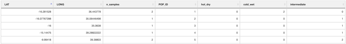
The built-in functions automatically select individuals that are falling within the range certain conditions following Razgour et al. (2019). For example, in a two predictor model (e.g. rainfall and temperature), certain individuals may be classed as ‘hot_dry’ or ‘cold_wet’ adapted. Individuals that fall in between the ordination categorisations of either of these categories may be categorised as ‘intermediate’. The distribution of these categorised individuals is plotted in the ordination space, and the function will collate the information for each individual, which category it belongs to, and its geographic location is saved in a separate .csv file. Categories (e.g. ‘hot_dry’/’cold_wet’) may be defined in the params file (‘category_1’, ‘category_2’).
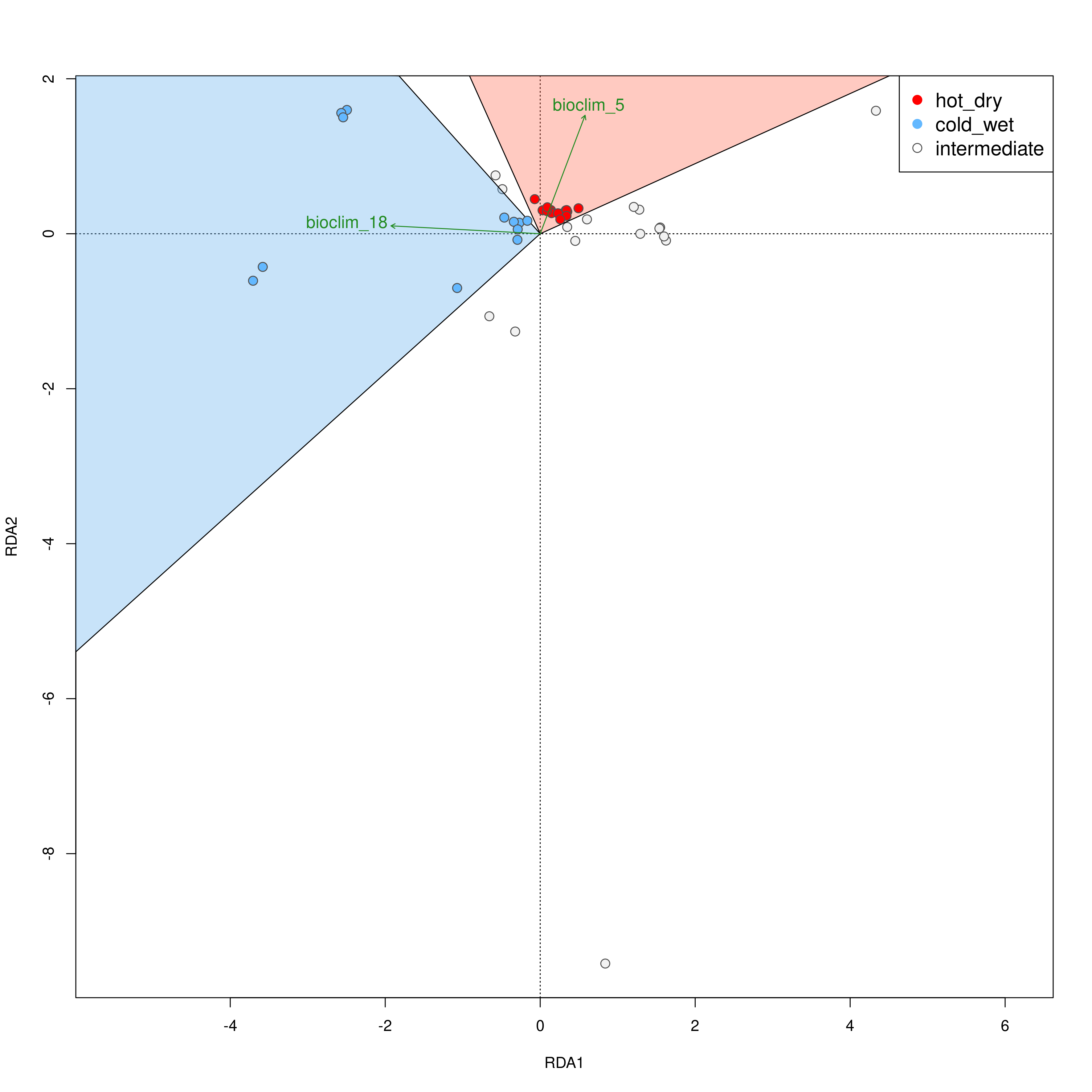
Individual categorisation
Hot-dry adapted individuals
Cold-wet adapted individuals
Intermediate individuals
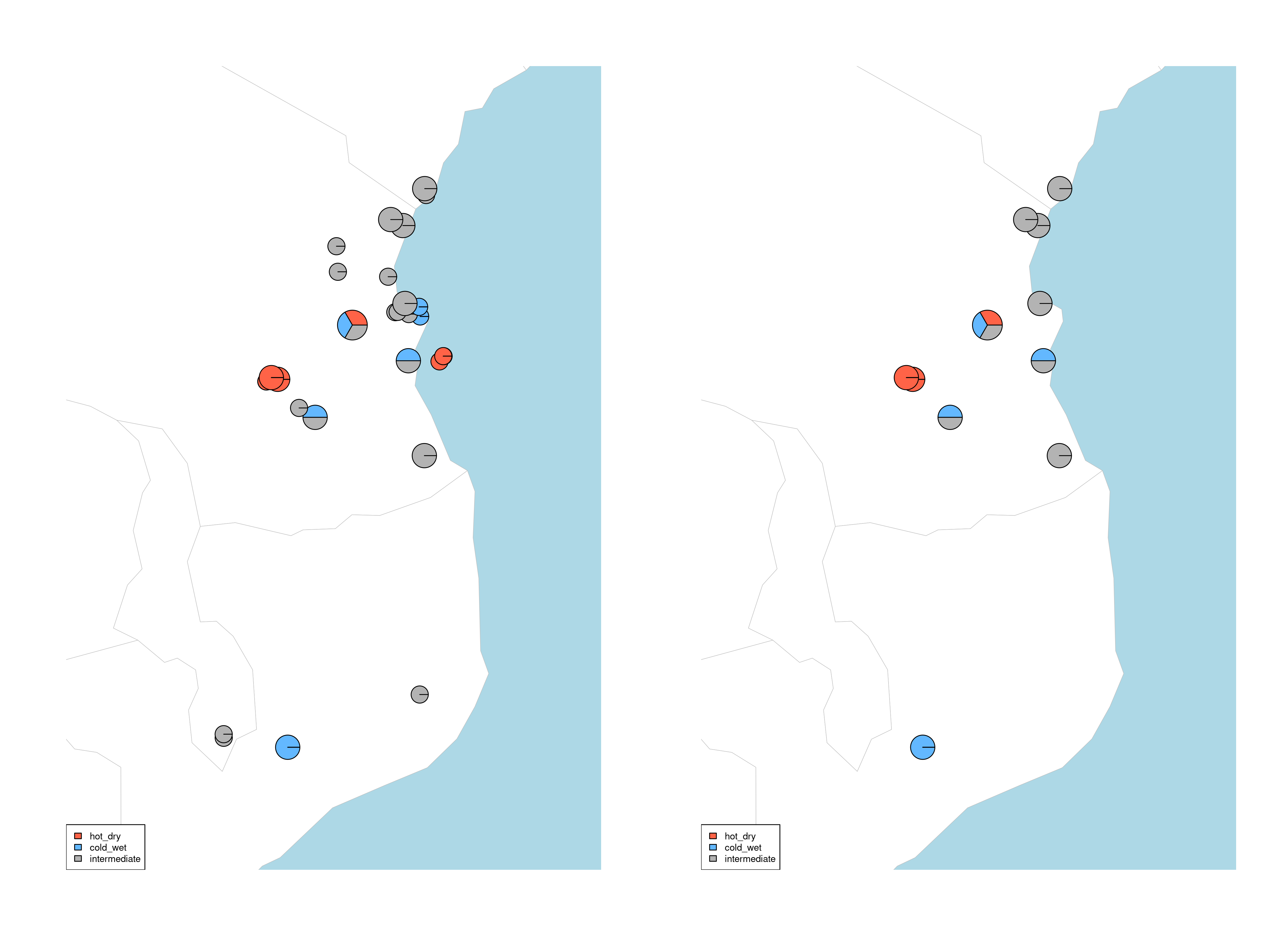
quantify_local_adaptations(species_binomial) will plot the local adaptation categories described above in geographic space. It plots the proportions of individuals that are adapted to each category defined in the params file (e.g. ‘hot_dry’/’cold_wet’/’intermediate’). It uses the outputs generated by the individual categorisation (above), and plots a summary map of all samples (individuals and populations) and which conditions they are adapted to
Summary of local adaptations across populations
Maps of local adaptations
genomic_offset(species_binomial) assesses population responses to future climate change based on their current vs. predicted future genotype-environment associations for a given climate scenario. We use genomic offsets, implemented in RDA using the approach of Capblancq and Forester (2021). For each population, a genomic offset value will be calculated based on the degree of local adaptation and the amount of predicted change in the future. The below plot shows what the output looks like, in our example the offset predictions are clipped to a buffer of 2 degrees around sampled localities to avoid predictions in geographic areas that are unreachable by the species. This can be modified in the params file with the ‘genomic_offset_buff_dist_degrees’ parameter.
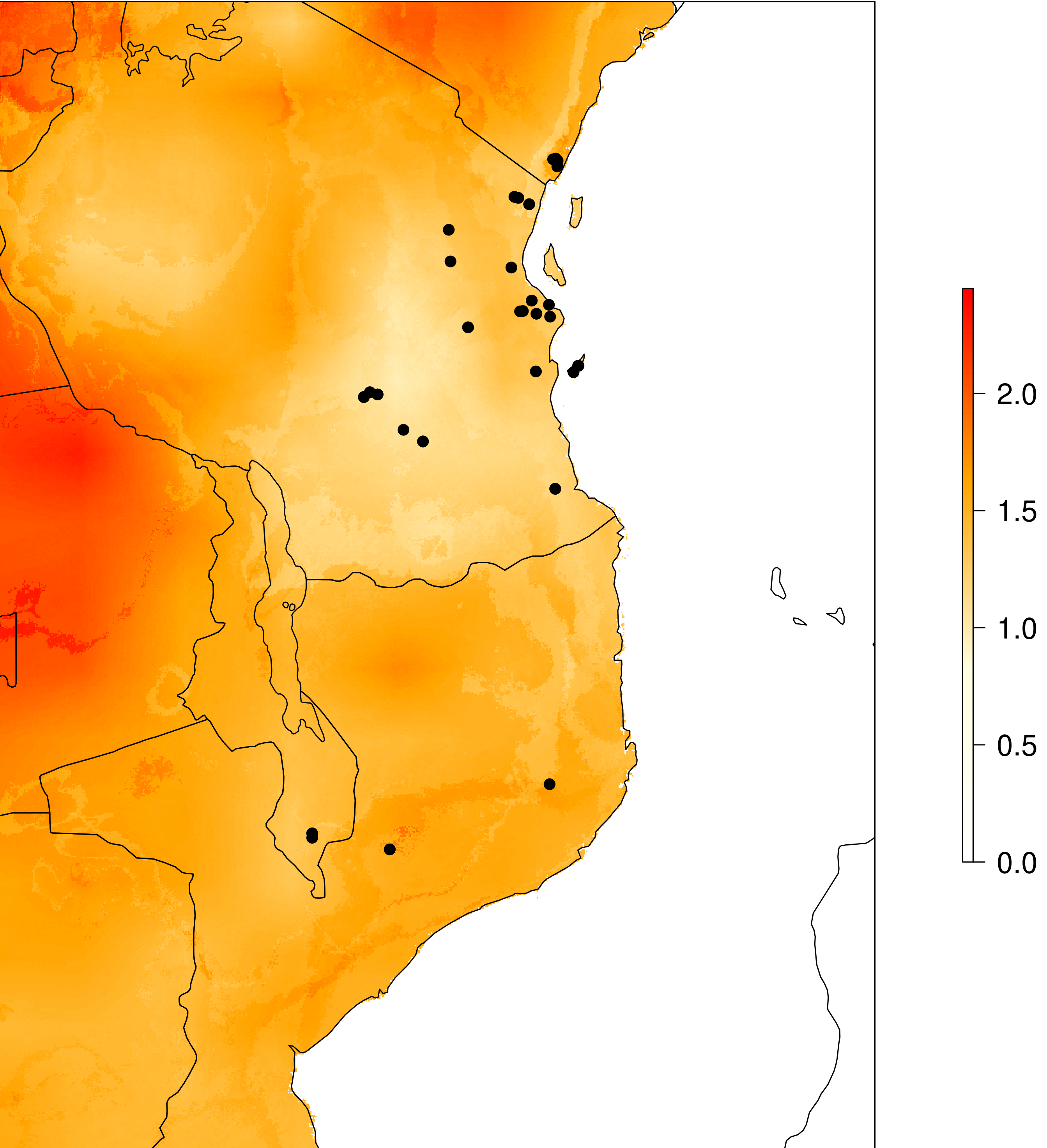
Genomic offset
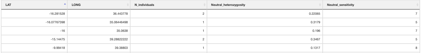
neutral_sensitivity() calculates neutral (i.e. non-adaptive) genetic diversity by masking out the putatively adaptive loci. It requires PLINK (Purcel et al. 2007) to be installed (read the binary location from the params file, ‘plink_executable’), then calls PLINK via R. PLINK will generate the output files and the script here will automatically count the populations, number of individuals and neutral nucleotide diversity to calculate ‘Neutral sensitivity’ (ranging from 1-10). Alternatively you may use heterozygosity instead of nucleotide diversity in your populations (for example if you have populations with only a single sampled individual then nucleotide diversity will return a value of 0 (NaN). If you want to use heterozygosity simply change the params file variable ‘neutral_sensitivity_metric’ to read ‘heterozygosity’ instead of ‘nucleotide_diversity’.
Summary of neutral sensitivity
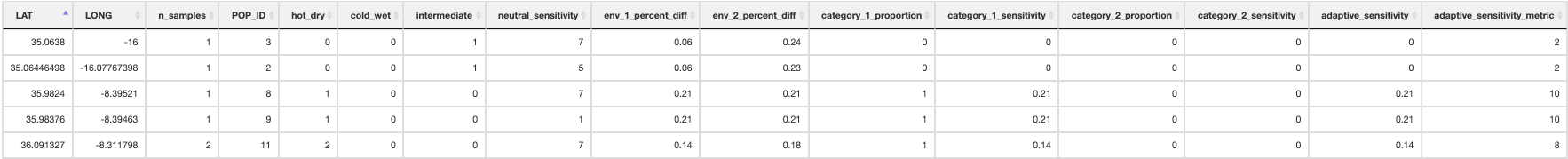
adaptive_sensitivity() uses the genomic offset values for each population to generate an ‘Adaptive sensitivity’ metric. The adaptive sensitivity metric will range between 1-10; being lower if a population has lower genomic offset, and higher with higher genomic offset.
Summary of adaptive sensitivity
create_circuitscape_inputs() will setup the necessary files and structure for the range shift potential analyses. Because the subsequent analyses will use Circuitscape to model pairwise connectivity, memory and time requirements can become substantial with large datasets (i.e many populations/localities). For this reason it is highly recommended that these are performed in a HPC environment. This script will write the required files (.ini, .jl) for Circuitscape to run in Julia, along with the necessary files (.sh) to submit these jobs via HPC. The script copies relevant files to the Circuitscape directory for analysis, and generates the specific required file for the spatial points input (derived from the input spatial genomic data), which is used to specify the ‘nodes’ to model connectivity between populations. In the params file, an option to transform all 0’s to values of 0.001 is provided (‘circuitscape_transform_zeros’) (recommended if running range shift potential analyses on SDM outputs) so that Circuitscape does not interpret unsuitable areas as completely impermeable barriers. Note that as mentioned in section 1, the parameterisation of circuitscape input resistance layers can be skipped if requested, but expects the necessary files in the correct places if you prepare this outside LotE. See section 14 for details.
11. Landscape barriers
To run the the Landscape barriers analyses (Circuitscape) run the following code embedded in a shell script:
julia --startup-file=no '$YOUR_WORK_DIR/-outputs-/Afrixalus_fornasini/Landscape_barriers/circuitscape/cumulative_circuitscape_layer.jl'
singularity exec ./bioconductor_3.14.sif Rscript ./-scripts-/run_LOE_Landsape_barriers.R 'Afrixalus_fornasini'
The circuitscape analyses will take a while to run, especially if there are many samples over a large geographic area (it will make pairwise comparisons across all sampling localities). The circuitscape analysis here models connectivity through the cumulative resistance surface (this has been parameterised using the ‘circuitscape_layers’ and ‘circuitscape_weights’ parameters in the Params.tsv file, though you can (and probably should) explore other possible drivers of gene flow such as environmental predictors, forest cover etc.). A widely used R package for optimizing resistance surfaces is ResistanceGA (Peterman, 2018).
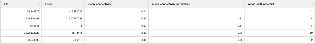
Once the Circuitscape analyses are complete, the R function Landscape_barriers() will automatically summarise and plot the data, as well as quantifying landscape barriers. landscape_barriers() reads in the output data from the Circuitscape analyses and plots maps of modelled current connectivity. It extracts the mean connectivity of each population to all other populations within a maximum dispersal distance (defined for each species in the params file) and then uses this to calculate ‘Landscape barriers’ (1-10), high landscape barriers = 10, low landscape barriers = 1. When calculating mean connectivity, a maximum dispersal distance in kilometres (‘max_dispersal_distance_km’) may be set in the params file for defining which populations are within geographic reach of one another (i.e. this avoids unrealistically distant populations being considered when calculating mean connectivity for each population).
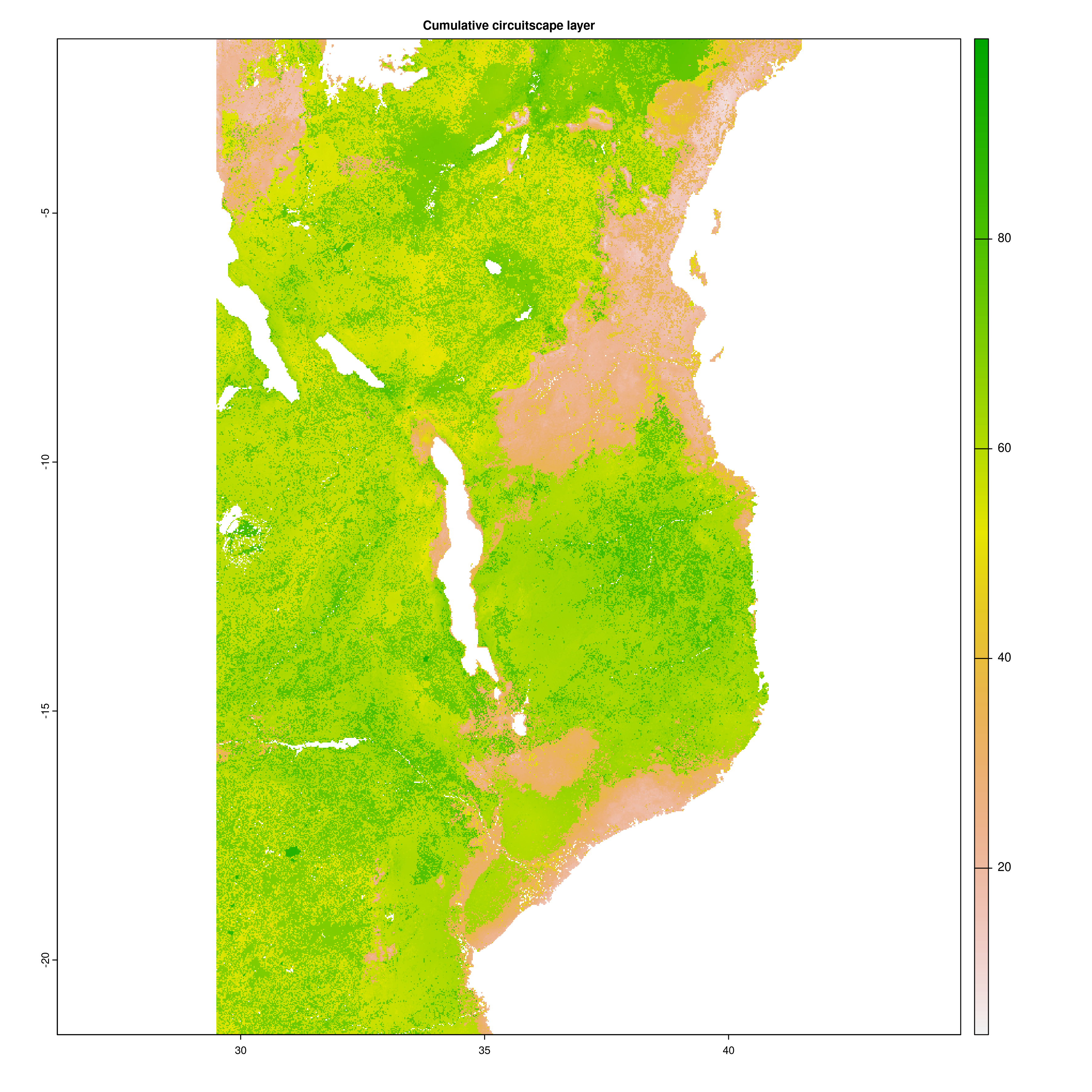
Circuitscape cumulative layer
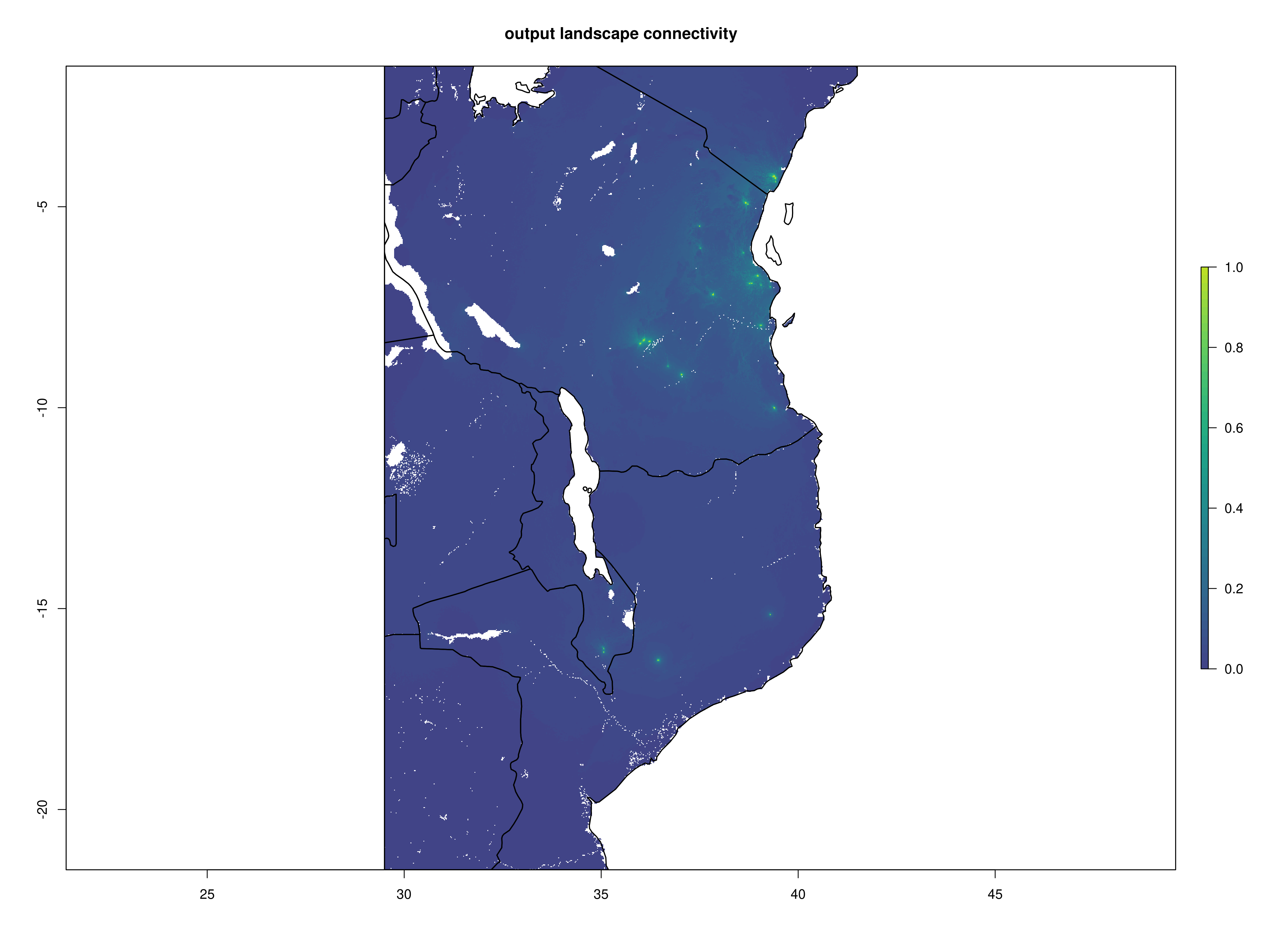
Landscape connectivity
Landscape barriers metric
12. Population_vulnerability
To run the final part of the toolbox, run the following code embedded in a shell script:
singularity exec ~/barratt_software/Singularity_container/bioconductor_3.14.sif Rscript ./-scripts-/run_LOE_population_vulnerability.R ‘Afrixalus_fornasini’
To elaborate the last part of this code, it will do the same as previously, running the population_vulnerability() function to create the final files, and then using summary_pdfs() will generate the final .pdf output which captures all the relevant outputs and information in a single pdf
population_vulnerability(species_binomial)
summary_pdfs(species_binomial)
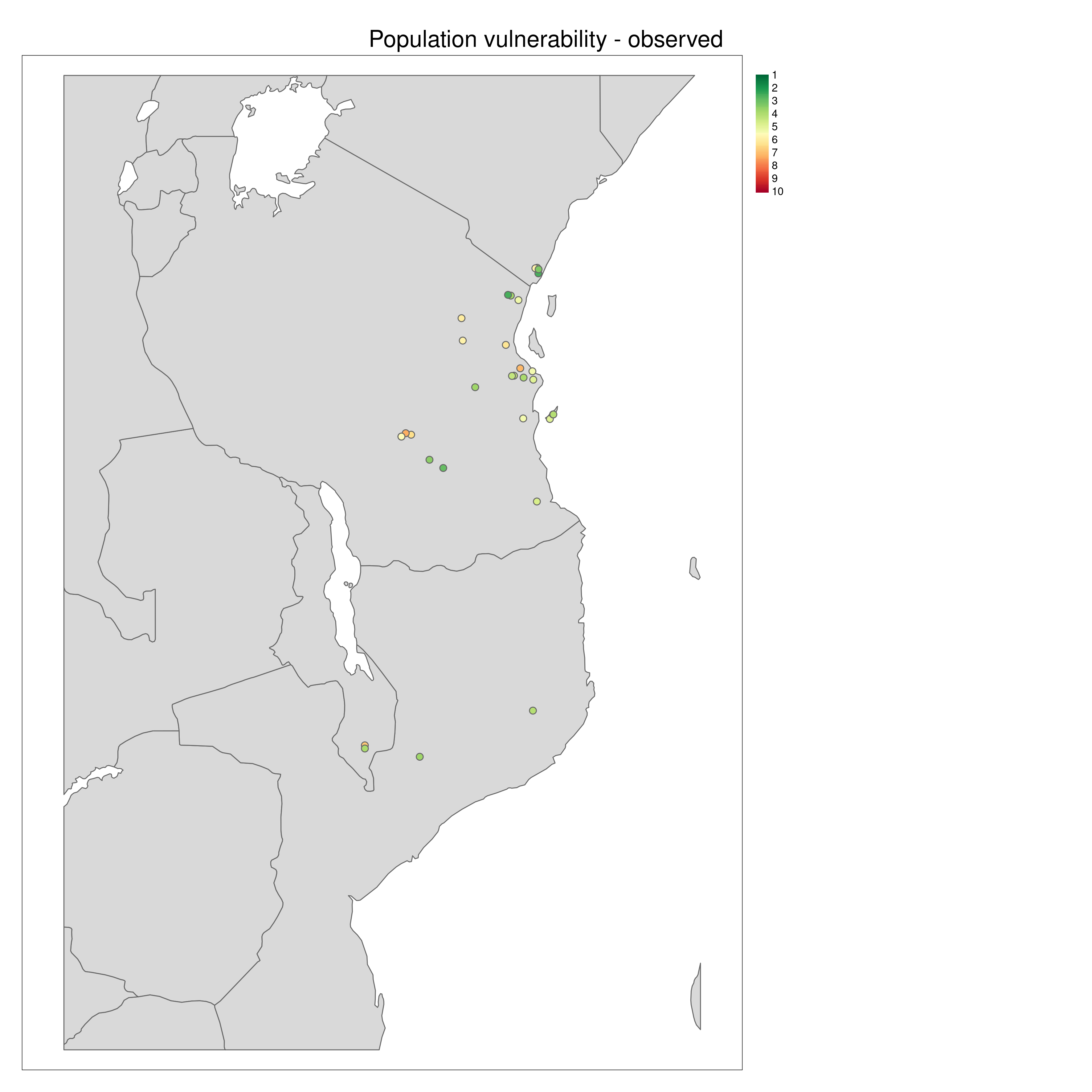
population_vulnerability() integrates the exposure, adaptive and neutral sensitivity and range shift potential results to create a summary ‘Population vulnerability’ metric per population ranging from low (0) to high (10). The function will create a .csv output file of the observed data (i.e. where genomic samples are located, and use an inverse distance weighted interpolation to predict Exposure, neutral sensitivity, adaptive sensitivity and Range shift potential results across geographical space, with the underlying assumption that locations closer together share similar properties than those further apart. The function produces summary maps of non-interpolated (observed) and interpolated (predicted) data for each of the metrics (separately and also a composite 4-panel map). To account for principles of complementarity between metrics, for each species that you analyse the composite 4-panel map of exposure, neutral sensitivity, adaptive sensitivity, landscape barriers will highlight the populations that are in the top 10% scores of the metric (highlighted by red circles) and the lower 10% of each metric (highlighted by green circles). This feature enables you to quickly identify population scores for each metric at a glance, so that relevant conservation actions may be considered. The params file allows the user to decide how population vulnerability is calculated by weighting the exposure, adaptive and neutral sensitivity and landscape barriers metrics
Population vulnerability
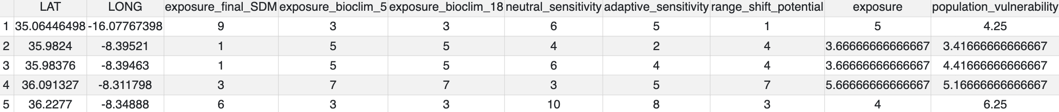
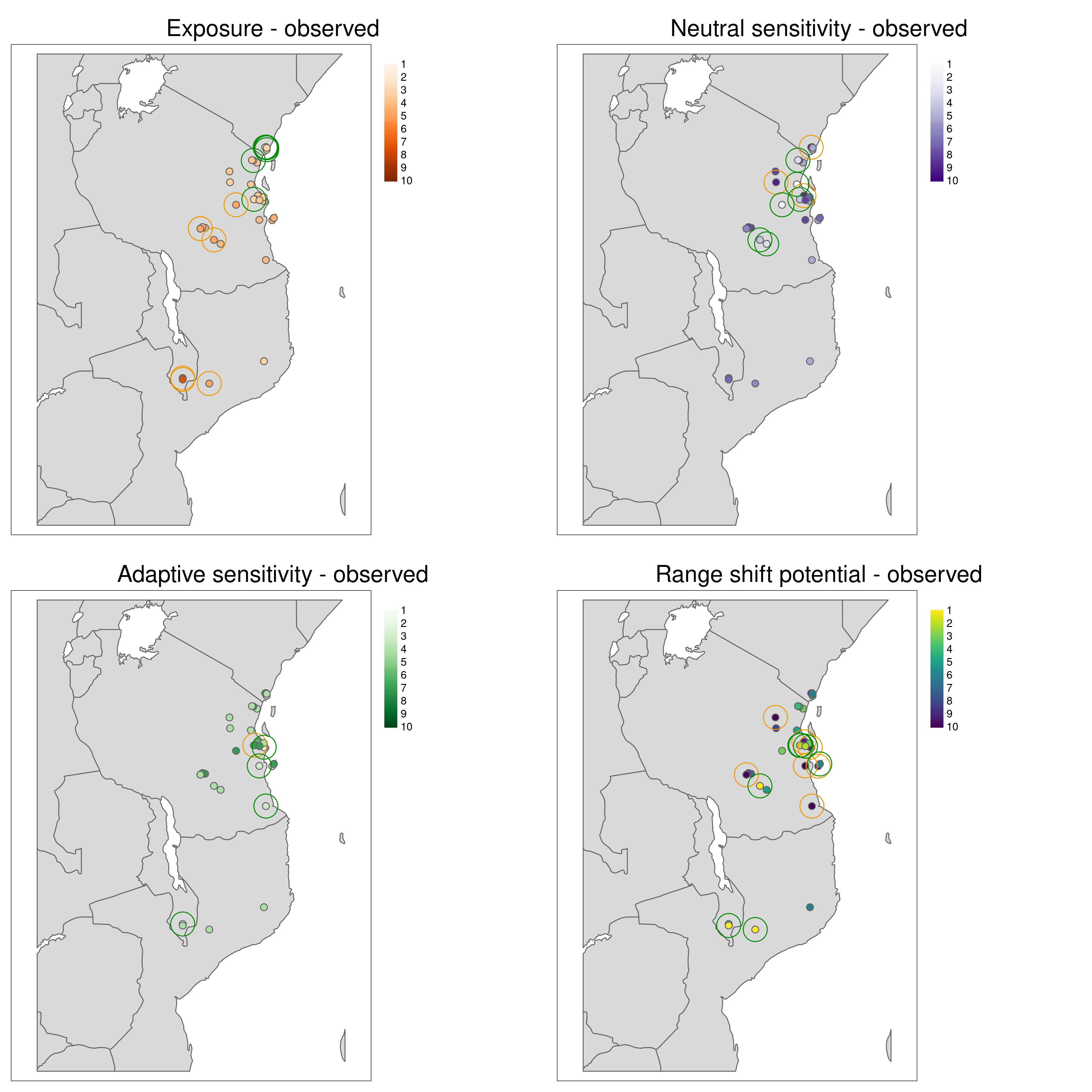
All metrics per population plotted in geographic space
Aligning with the concepts of complementarity in conservation, LotE will also provide plots of the highest and lowest ranked metrics (Exposure, Neutral sensitivity, Adaptive sensitivity, Landscape barriers, see images below) per population so that the user can gain a sense of differences between the metrics for each population. For example, a population with high landcape barriers and high exposure may benefit from assisted migration, whereas a population with low landscape barriers and low adaptive sensitivity may benefit from habitat restoration along connectivity corridors.
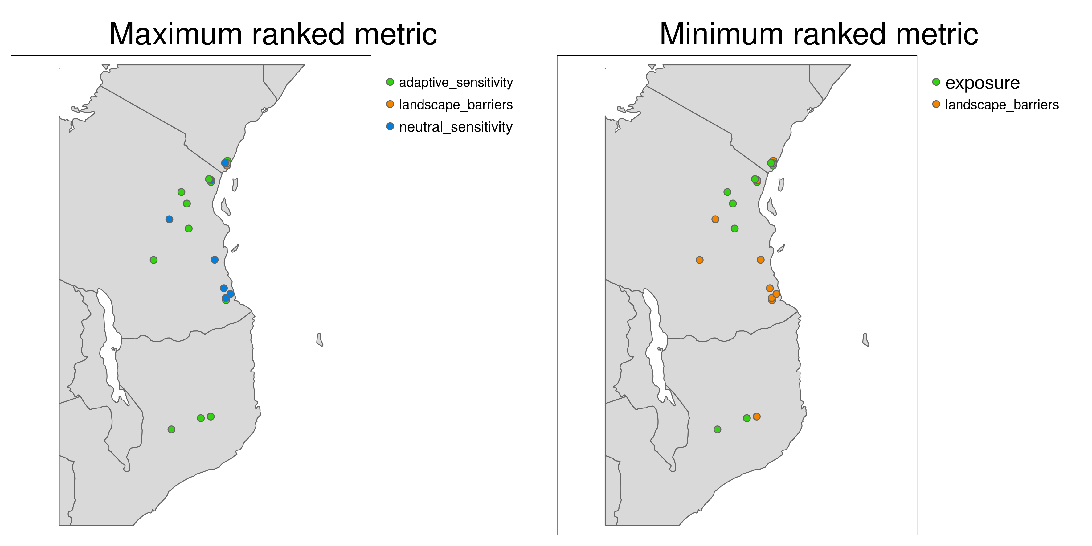
*Maximum and minumum ranked metrics per population**
Population vulnerability
summary_pdfs() uses all outputs generated and information in the log file to paste results together into a final summary PDF sheet using the grobblR package (Floyd, 2020). The contents of the final summary PDF will depend if you have run the full LotE toolbox - if you have skipped certain steps as detailed in section 1 (e.g. SDMs, GEAs, imputing genotypes, circuitscape parameterisation) then these parts will be replaced with the inputs you provided. Results can be identified and probed by rerunning the individual functions with modified parameter settings, and we recommend thorough reporting and transparency in all publications that use this toolbox.
13. Skipping tricky parameterisations
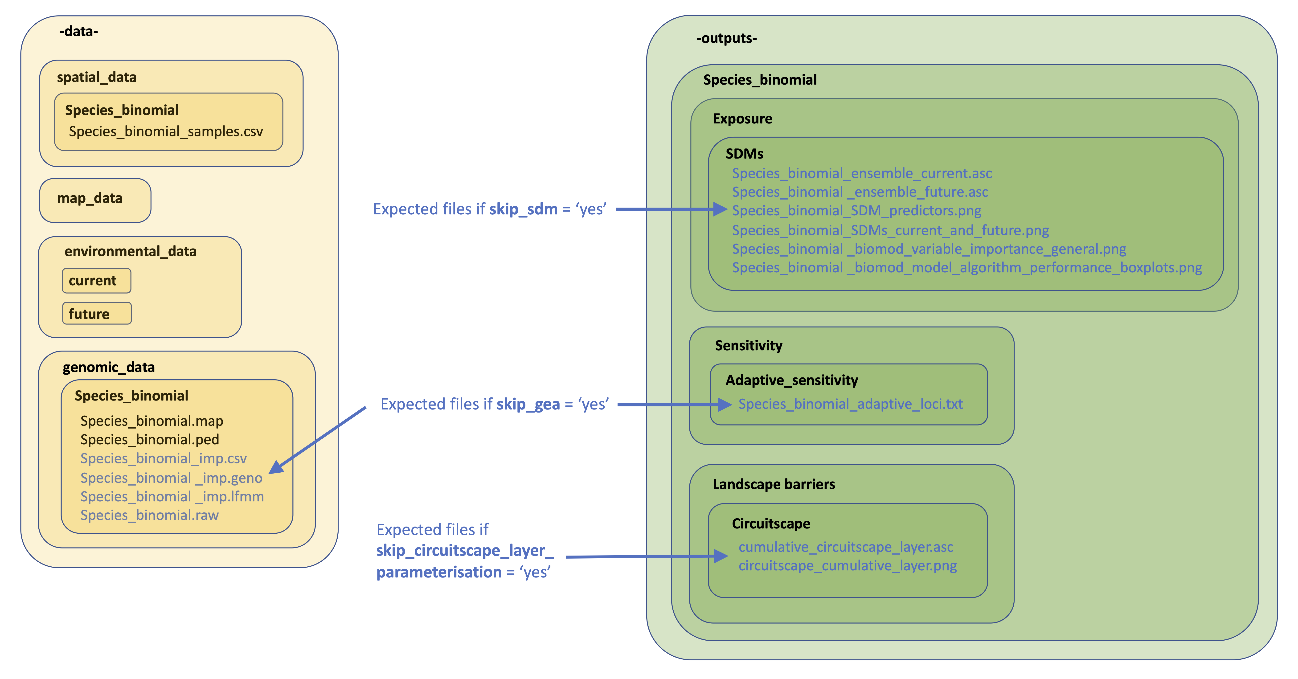
The below image provides details on the files expected by LotE if you decide to skip the relevant parts of the toolbox (e.g. skip_sdm, skip_impute_genotypes, skip_gea, skip_circuitscape_layer_parameterisation options). If you want to prepare these analyses outside the toolbox with the help of an expert or a different piece of software (e.g. Maxent for SDMs, MACH for genotype imputation, Baypass for GEAs, or ResistanceGA/radish for parameterising a Circuitscape resistance surface), you’d need to make sure the directory structure is as below, especially ensuring already creating directories and subdirectories as indicated. Blue text are files you will need to add. Examples of all of these and their formats can be found here
File requirements if skipping certain sections of LotE
14. Running multi-species analyses
One of our main motivations for developing LotE was so that multiple datasets of suitable matching georeferenced genomic data can be analysed following the same underlying framework that is standardised and reproducible. In principle, all you require are the genomic data themselves (.ped, .map format) and the spatial coordinates of the samples within these files, saved as a .csv format file. Once you have collected the data together you can simply have a new line for each species name (species_binomial) in the params file, and off you go!
Before you do this however, there are a few things that need to be considered first. Do you aim to compare species results with one another directly? If so, you need to think about how you will generate the exposure, neutral sensitivity, adaptive sensitivity, Landscape barriers and population vulnerability metrics. Making direct comparisons can be relatively straightforward as long as the species are ecologically/evolutionarily similar (e.g. several closely related species within a genus with a shallow divergence time). In this case you could define the way the metrics are quantified in the params file to be the same across all species you compare (e.g. set exposure_quantification, neutral_sensitivity_quantification, adaptive_sensitivity_quantification, landscape_barriers_potential_quantification and population_vulnerability_quantification to ‘defined’, and set exposure_thresholds, neutral_sensitivity_thresholds, adaptive_sensitivity_thresholds, landscape_barriers_thresholds and population_vulnerability_thresholds to e.g. ‘1,2,3,4,5,6,7,8,9,10’).
However, an approach like this may be slightly complicated if your species are not closely related (e.g. millions of years divergence and in separate genera/families) because they likely have very different evolutionary and ecological constraints (e.g. thermal tolerances, levels of genetic diversity, and many more factors). If you do compare multi-species that are very different like this we recommend that instead of directly comparing metrics between species, that you instead aim to highlight the areas across the species range where metrics of interest (e.g. overall population vulnerability) are highest and then compare these across species qualitatively rather than direct comparison of metrics which are generated from very different underlying datasets. This can be done by identifying the lowest and highest metrics that a population represents for example, which is also automatically generated by LotE.
15. Understanding analyses (and skipping those that you are not comfortable with…)
If you are not confident in parameterising certain analyses, we strongly recommend that you bring someone onboard that is. In particular, SDMs should be well parameterised as well as GEAs (LFMM and RDA), for which you’ll likely need to impute missing genotype data. The processing of genomic data, particularly RAD-seq style data, is also riddled with potential pitfalls (see here for an overview), so you’ll need to have someone that understands the inherent biases in these datasets, and how they can be mitigated. Lastly, parameterisation of resistance surface inputs for circuitscape can be complex. You can skip the parameterisation of these steps in particular using the skip_sdm, skip_impute_genotypes, skip_gea, skip_circuitscape_layer_parameterisation options. If any of these are set to ‘yes’ in your params file for a given species, these steps will be skipped. If you want LotE to run to completion (i.e. to obtain population vulnerability and summary PDFs) you’ll need to supply the missing files that LotE is expecting. A guide to this is found in section 13 above.